Um novo estudo sugere que entre os adolescentes os distúrbios de saúde mental podem ser “transmitidos socialmente”, embora os seus investigadores não tenham conseguido estabelecer qualquer causa direta. Carol Yepes por meio do Getty Images
A natureza contagiosa das infecções bacterianas ou virais, como infecções na garganta ou gripe, é bem compreendida. Você corre o risco de pegar gripe, por exemplo, se alguém próximo a você a contrair, pois o vírus pode se espalhar por meio de gotículas no ar, entre outros modos de transmissão. Mas e a saúde mental de uma pessoa? A depressão pode ser contagiosa?
UM Psiquiatria JAMA artigo publicado no início deste ano parecia sugerir isso. Os pesquisadores relataram ter encontrado “uma associação entre ter colegas diagnosticados com transtorno mental durante a adolescência e um risco aumentado de receber um diagnóstico de transtorno mental mais tarde na vida”. Eles sugeriram que, entre os adolescentes, os distúrbios de saúde mental poderiam ser “transmitidos socialmente”, embora o seu estudo observacional não tenha conseguido estabelecer qualquer causa direta.
Faz algum sentido intuitivo. Os psicólogos estudaram como o humor e as emoções podem se espalhar de pessoa para pessoa. Alguém uivando de tanto rir pode ser contagioso, no sentido de que também faz você rir. Da mesma forma, ver um amigo com dor emocional pode evocar sentimentos de desespero – um fenômeno denominado contágio emocional.
Durante mais de três décadas, os investigadores investigaram se as perturbações de saúde mental também podem ser induzido pelo nosso ambiente social. Estudos encontraram resultados mistos sobre até que ponto amigos’, pares’ e famílias‘a saúde mental pode, por sua vez, impactar a saúde mental de um indivíduo.
O Psiquiatria JAMA Um estudo – conduzido por pesquisadores da Universidade de Helsinque, na Finlândia, e de outras instituições – analisou dados de registros nacionais de 713.809 cidadãos finlandeses nascidos entre 1985 e 1997. A equipe de pesquisa identificou indivíduos de escolas de toda a Finlândia que haviam sido diagnosticados com um transtorno mental no momento em que nasceram. na nona série. Eles seguiram o restante da coorte para registrar diagnósticos posteriores, até o final de 2019.
O estudo descobriu que os alunos do nono ano que tiveram mais de um colega diagnosticado com um transtorno de saúde mental tiveram um risco 5% maior de desenvolver uma doença mental nos anos subsequentes do que os alunos sem nenhum colega com diagnóstico. O risco foi particularmente elevado no ano imediato após a exposição: os alunos com um colega diagnosticado tinham 9% mais probabilidade de receber um diagnóstico de saúde mental, enquanto os alunos com mais de um colega diagnosticado tinham 18% mais probabilidade de receber um diagnóstico. O risco foi maior para transtornos de humor, ansiedade e alimentares. Foi observado um risco aumentado após o ajuste para uma série de possíveis fatores de confusão a nível parental, escolar e regional, como a saúde mental dos pais, o tamanho das turmas e as taxas de desemprego ao nível da área.
Estes resultados podem parecer provas convincentes da transmissão social de perturbações de saúde mental, mas outros investigadores – como Eiko Fried, psicóloga clínica da Universidade de Leiden, nos Países Baixos – sugeriram que a equipa finlandesa pode não ter controlado todos os fatores de confusão relevantes. Fried mencionou morar em um bairro pobre, o que aumenta o risco de depressão, como exemplo de um fator de confusão em um e-mail para Escuro. “Essas crianças acabam nas mesmas escolas, e há um acúmulo de depressão nessas escolas. Isto agora parece um contágio social, até que o fator de confusão – a vizinhança – seja levado em conta.”
Os investigadores controlaram as taxas de emprego e os níveis educacionais dos bairros, mas é possível que ainda não tenham levado em conta outros factores contextuais influentes. Na medida em que estes factores partilhados são medidos de forma insuficiente, as estimativas de resultados correlacionados correm o risco de atribuir a causalidade à variável errada. Em um publicar no X (antigo Twitter), Fried disse que pode ser mais plausível que fatores de confusão ocultos expliquem o que está acontecendo, em vez de contágio social.
Em resposta a uma consulta por e-mail que apresentava críticas sobre variáveis potencialmente confusas, o principal autor do estudo finlandês, Jussi Alho, sublinhou a utilidade de utilizar as salas de aula como ponto de referência, apontando para outra influência potencial: a tendência das pessoas procurarem ou ser atraído por aqueles que são semelhantes a eles. “Em nosso estudo, mitigamos esse viés de autosseleção usando aulas escolares como proxies para redes sociais”, explicou. “Como redes sociais impostas institucionalmente, as turmas escolares são bem adequadas à investigação, uma vez que normalmente não são formadas endogenamente por indivíduos que selecionam outros semelhantes como colegas de turma. Além disso, as aulas escolares estão indiscutivelmente entre as redes de pares mais significativas durante a infância e a adolescência, dado o tempo substancial passado junto com os colegas de classe.”
Pelas contas de Alho e dos seus co-autores, tal como escrevem no artigo, a força do estudo finlandês reside no facto de as redes sociais investigadas não terem sido escolhidas de forma independente pelos sujeitos da investigação. Ao mesmo tempo, Alho admitiu que os críticos têm razão: “Não podemos descartar totalmente a possibilidade de confusão residual”, escreveu ele num e-mail para Escuro“devido a covariáveis não medidas ou medidas incorretamente em nosso estudo”.
Esses fatores de confusão são um problema persistente que persegue esta linha de pesquisa. Um 2012 estudar publicado na revista Economia da Saúdepor exemplo, examinou o estado de saúde mental de estudantes universitários colegas de quarto durante o primeiro ano, testando o possível “contágio entre pessoas que são colocadas juntas em grande parte por acaso”. Os autores descreveram o estudo como um experimento naturalque argumentaram que seria capaz de produzir, nas suas palavras, “estimativas imparciais” de “efeito causal”.
Os investigadores não encontraram “nenhum contágio global significativo para a saúde mental e apenas pequenos efeitos de contágio para medidas específicas de saúde mental”, como sofrimento psicológico geral, depressão e ansiedade. Mesmo neste caso, porém, o ligeiro efeito de contágio pode ser atribuído a factores não medidos, como o facto de os estudantes partilharem ambientes sociais e formações comparáveis. Afinal, eles estão frequentando uma escola que poderiam ter escolhido com base em interesses acadêmicos ou habilidades extracurriculares semelhantes.
Todas essas possíveis influências tornam difícil saber o que está motivando o quê. Os problemas de saúde mental estão se espalhando entre as pessoas nas redes sociais? Ou estarão alguns outros factores desconhecidos apenas a criar essa impressão?
Qualquer que seja a resposta, essas exposições pessoais podem estar a provocar um tipo diferente de contágio: conscientização pública. O transtorno de ansiedade generalizada, por exemplo, apareceu pela primeira vez como diagnóstico na terceira edição do Manual Diagnóstico e Estatístico de Transtornos Mentais (DSM) em 1980. A condição causa “preocupação excessiva, frequente e irreal com as coisas do dia a dia”, de acordo com o Biblioteca de Saúde da Clínica Cleveland. Quando a quarta edição do DSM e seus critérios diagnósticos atualizados para transtorno de ansiedade generalizada foram lançados em 1994, o transtorno havia “se transformado de uma condição raramente diagnosticada em um transtorno com prevalência ao longo da vida atingindo até 5% em uma amostra da comunidade”. de acordo com um artigo de 2017 na história do diagnóstico. Dados de uma Agência de Pesquisa e Qualidade em Saúde de 2016 relatório sobre ansiedade em crianças indica que a ansiedade infantil ocorre em aproximadamente uma em cada quatro crianças com idades entre 13 e 18 anos, enquanto a prevalência ao longo da vida de transtorno de ansiedade grave nessa faixa etária é de 5,9 por cento.
O que está causando essas taxas é uma conscientização potencialmente melhor entre pacientes e médicos. Ou pode resultar de uma série de outros factores, como a evolução dos critérios de diagnóstico e a melhoria do acesso ao tratamento. Mas, como Alho e os seus colegas sugerem no seu artigo, é possivelmente também impulsionado pelo conhecimento e aceitação dos distúrbios de saúde mental obtidos através das redes sociais. Afinal de contas, estar exposto a um colega com uma perturbação mental, observaram os investigadores no seu estudo, pode muito bem ajudar na “normalização das perturbações mentais através de uma maior consciência e receptividade ao diagnóstico e tratamento”.
Joshua Cohen é analista independente de saúde e escritor freelancer baseado em Boston, e autor de Escurode Seções transversais coluna.
When the sun sets, darkness guides the ways many animals live and die. The night helps wary mice hide from some predators, but it also helps hunters like keen-eyed owls score their next meal. Many species mate under cover of darkness, like calling crickets that find one another in the night. Animals from seals to dung beetles rely on the stars or moon in dark skies for navigation. The cycling of day and night creates a natural clock that enables a restorative night’s sleep for primates like us. When the days shorten, changes in light help ready hibernators for seasonal slumber or cue migrating monarch butterflies that it’s time to fly.
“There’s an entire evolutionary history of predictable patterns of light and dark,” says Travis Longcore, an environmental scientist at the University of California, Los Angeles, and co-editor of the book Ecological Consequences of Artificial Night Lighting.
But now that artificial lighting has exploded around the globe, it’s having enormous impacts. Purple martins are migrating earlier in the spring, as the birds’ seasonal clocks are confused by artificial light. Artificial light exposure lowers levels of melatonin, a hormone that helps regulate sleep cycles, in dozens of species, adding stress and depriving them of a good night’s rest. “Wherever you look you’re going to find influences, because we’ve just so profoundly changed what the natural rhythms are to artificial rhythms,” says Longcore.
Research into the many ways artificial light at night influences creatures has exploded in recent years. We searched across the animal kingdom to spotlight 11 examples of how street lights, porch lights, illuminated buildings and more dramatically affect animal behavior.
Spider brains shrink in the spotlight
When faced with artificial light exposure, Australian garden orb-weaving spiders suffer dwindling volume in a brain region linked to their vision, according to a September study in Biology Letters.
Spider brains aren’t centralized like ours. They consist of distinct structures linked together, which makes it easier to see changes to specific regions and, potentially, the functions they govern. The University of Melbourne’s Nikolas Willmott and colleagues recently used micro-CT scans to spot brain shrinkage when the spiders were exposed to light at night.
Willmott theorizes that the stresses of artificial light may lead them to reallocate resources into more important parts of the brain. Or, he suggests, the light might disrupt hormonal processes in that part of the brain, which in turn stunts its growth and development.
Willmott hopes future research can provide a better understanding of the mechanisms driving these artificial light effects on the arachnid brain, and whether light could even produce physical changes like eye size. “There is still a lot that we don’t know,” he says.
City lights lead birds astray
Lights Out: Philadelphia Darkens Its Skyline to Protect Migrating Birds
Hundreds of bird species migrate in the dark, when the air is cool and predators few, following the moon and stars along ancient routes. But dazzling arrays of unfamiliar lights have appeared along the way. Urban buildings and towers often disorient birds, and for unknown reasons even attract them, causing the birds to crash or circle confusedly until they succumb to exhaustion. Millions of birds die this way, a problem of such scale that Philadelphia, Chicago, San Francisco and other cities have adopted “Lights Out” initiatives during migration periods, when unnecessary lights are dimmed or simply turned off.
Mining, hydrocarbon extraction, fishing and other industries also produce lots of artificial light in places with few people. And skyglow from artificial light often causes migrating birds to linger where they normally wouldn’t, disrupting their annual trips. “We know now from the work that’s been done on birds we are literally changing the places birds migrate across continents,” Longcore says.
Light pollution also hurts birds by altering their biological clocks. Birds at overwintering sites may mistake artificial light for the longer periods of daylight that alert them to the coming of spring. This could spur early migrations, when ideal temperatures and food along their routes may not be available.
Illumination can ruin coral reproduction
The global atlas of artificial light in the sea reports that biologically significant levels of artificial light pollution penetrate to depths of at least three feet across 735,000 square miles of the ocean. That affected area is about the size of Mexico.
Light pollution has impacts offshore, where research shows that it may hinder coral reproduction. Many corals reproduce just once a year during a period of darkness in the days after a full moon. The synchronization has taken place over countless generations. Each individual coral releases eggs or sperm simultaneously, creating the best conditions for fertilization success, genetic diversity and protection from predators—which simply can’t consume all the eggs.
But research shows that artificial light, particularly LED lights rich in the same blue wavelengths as moonlight, can throw off this intricate dance and trigger corals in the same locations to spawn at different times. This may disrupt reproduction in an era when corals are in serious decline and face a plethora of other threats like rising water temperatures and destructive diseases.
Lights can send baby sea turtles down dangerous paths
Saving Sea Turtles with Wildlife Friendly Lighting
Sea turtles spend years at sea and migrate thousands of miles, but when it’s time for females to lay eggs, they depend on nesting beaches and often return to the same location. These coastal areas are also desirable for humans, who have developed many of them and inundated areas with nighttime illumination.
Artificial lights hinder sea turtle nesting success in multiple ways. They discourage female turtles from returning to historical nesting beaches—making them choose less successful locations simply because they are dark. Worse, young turtles hatch at night, when predators are scarce. Light from the moon and stars in the night sky reflects on the ocean and guides the hatchlings to the water. But hatchlings are also attracted by bright artificial lights and may follow them inland, where they become exhausted and dehydrated, or fall prey to birds or other predators. Research also shows that even those hatchlings that reach the ocean can be attracted by artificial lights on the water, which can prevent them from successfully dispersing.
Artificial lights fragment bat habitat
A recent study of North American bat species tracked their reactions to the LED lights typically found in backyards and on garages. Little brown bats avoided the lights entirely to distances of at least 250 feet—where human eyes can no longer even notice the glow. This light aversion, shared by big brown bats, may eliminate many roosting locations and reduce or fragment the crucial habitat they use for feeding. Other species, like eastern red bats, did not seem to mind lights and may feed on insects drawn to the glow.
Scientists first started observing how streetlights disturbed commuting bats 15 years ago and found out that some species seemed hard-wired to avoid the lights. Such research illuminated a problem: Evaluating ecosystems during the day misses how important factors like artificial light affect animals when most humans are indoors or asleep. “If you don’t think of conservation planning from the nighttime view as well, you’ve haven’t really done it,” Longcore says. Light pollution’s impacts also vary by environment. For example, when well-lit areas also feature trees, bats do better, German researchers learned.
Human lights silence fireflies flashing “language”
Fireflies light up the night in Taiwan.
I-Hwa Cheng / AFP via Getty Images
Artificial light creates a unique set of problems for creatures like fireflies that produce their own light.
Fireflies light up a field or backyard as a form of communication. Among their 2,000-odd, species the language-like function of the flashing can vary dramatically. Some light up when threatened, or when trying to lure prey. Flashes often send mating messages, projecting key information like sex and species to attract suitable partners.
Artificial lights at night affect the ubiquitous American toad during various phases of its life cycle. An Ohio study examined tadpoles of the species from 40 artificial ponds; half exposed to small amounts of artificial light at night and the others left naturally in the dark. All the tadpoles became toads, but those from light-exposed ponds were 15 percent smaller. Researchers theorize that toads exposed to artificial lights at night burned energy by being active while the others rested.
Studies of Europe’s common toad also show that light can shut down activity—and confound mating efforts. French scientists exposed dozens of breeding males to various levels of nighttime light that mimicked natural moonlight, the glow of a streetlight or the floodlit landscape of an urban park. Toads exposed to streetlight conditions were 56 percent less active, while those in well-lit park conditions saw normal activity reduced by 73 percent. These toads may reallocate energy from activity to dealing with the stress of light exposure. The males exposed to artificial light also took longer to find mates, and those exposed to the streetlight intensity were 25 percent less likely to successfully fertilize a female.
Wallaby moms may delay births due to lights
The presence of artificial lights may lead tammar wallabies to give birth later than usual.
JOUAN / RIUS / Gamma-Rapho via Getty Images
Tammar wallabies—small, kangaroo-like mammals from Australia—mate in October, part of the Southern Hemisphere’s spring. Females hold their embryos dormant until after December’s summer solstice then, as each day gets a bit shorter, deliver babies in late January.
But researchers near Perth compared populations living in natural darkness with those around a well-lit naval base. Moms living near the base’s lights apparently missed the cues of shortening days and delivered their babies a full month later. These moms produced far less melatonin, a hormone that helps regulate their cycles of sleep and wakefulness, and this may have helped delay the timing of births.
Researchers can’t say yet how this change might influence the wallabies’ survival, but serious problems are possible when species’ reproductive timelines get out of sync with seasonal weather conditions and food availabilities. “If you’re a species that depends on a seasonal resource,” Longcore explains, “you have to have signals that get you to that resource at the time when you need it.”
Spawning grunion shun the spotlight
In spring and summer, during the few days following a full moon, teeming grunion pack the shorelines during dramatic spawning runs. The fish beach themselves to lay, fertilize and bury eggs. After a week or so, the young hatch at high tide and head to sea.
But research reveals that on shorelines where artificial light creates a glow equivalent to that of a full moon or more, the fish are far less likely to run.
“You can basically predict where you’re going to have a good grunion run, based on the level of light,” Longcore says. Why do the fish avoid the spotlight? “I think it turns them into a buffet for the predators,” he says. “There are plenty of records of birds just sitting there and picking off the grunion.”
Artificial light aids cannibal crabs
The eternal dance between predators and prey plays out during the cycles of light and dark. Darkness can help some species avoid being eaten. So night lights can help predators more easily spot prey—including their own kind.
Consider the South American intertidal burrowing crab, a key species in the tidal flats and salt marsh grassland ecosystems of coastal Brazil and Argentina. Scientists ran an experimental study to see how artificial lights affected the ability of juvenile crabs to survive. Juvenile survival among crabs living near low-power LED lights was 61 percent lower than those living under natural dark conditions. One reason why? Light increased the incidence of cannibalism. Crabs living under natural conditions had a 30 percent better chance of avoiding being eaten by adult males of their own species, which were five times more abundant in lit areas.
Moths drawn to artificial lights succumb to exhaustion
Thousands of moths swarm a light at a stadium in Australia.
Fairfax Media via Getty Images
Why are insects irresistibly drawn to a light? Some scientists suggest heat is the attractant, while others believe the light is misinterpreted as a hole or passage.
But a study earlier this year may have answered the question: It suggests that many insects orbit around a light because they mistakenly believe they are orienting themselves by sky light. The authors observed that moths, dragonflies and other flying insects kept their backs continuously tilted toward the light as they moved, apparently believing it to be bright sky above them, contrasted with the dark ground below. “Flying animals need a reliable way to determine their orientation, especially relative to the direction of gravity,” lead author Samuel Fabian, a bioengineer at Imperial College London, explained in a press release.
Unfortunately, this behavior locks bugs into awkward orbits around artificial lights that eventually lead to exhaustion or crash landings. Turning off unneeded lights is a good way to reduce this carnage. But more necessary artificial lights that are left on will still have impacts, including many that are yet to be discovered. “A key next step for this research is to work out how distance changes the effect of lights at night,” Fabian said. “We know what’s happening at one meter from a light, but what’s happening at 100 meters?”
A análise do Bullet Cluster, que se formou após a colisão de dois grandes aglomerados de galáxias, apoia a existência de matéria escura. Raio X: NASA/CXC/CfA/M. Óptica: NASA/STScI; Magalhães/U. Arizona/D. Clowe et al.; Mapa de lentes: NASA/STScI; WFI do ESO; Magalhães/U. Arizona/D. Clowe et al.
O universo é composto de muito mais do que aparenta. Embora os telescópios revelem inúmeras galáxias, cada uma contendo milhares de milhões de estrelas, os físicos e astrónomos acreditam que a matéria visível é apenas a ponta do iceberg, por assim dizer, e que algum tipo de galáxia invisível matéria escura também deve estar lá fora, representando cerca de 85% da massa do universo. Ninguém sabe do que é feita a matéria escura, mas os cientistas estão confiantes de que é algo que não interage com a radiação eletromagnética, como a luz – caso contrário, seríamos capazes de vê-la. Mas décadas de pesquisas não conseguiram produzir qualquer deteção direta desta matéria escura, deixando os investigadores a questionarem-se se precisam de alargar as suas estratégias de pesquisa, ou talvez até de repensar como funciona a gravidade.
A defesa da existência de matéria escura remonta à década de 1930, quando os astrónomos analisaram as taxas de rotação das galáxias e descobriram que não havia matéria visível suficiente para explicar as taxas de rotação observadas. Esses chamados curvas de rotaçãoque traça a velocidade com que as estrelas se movem em função da distância ao centro de uma galáxia, não pôde ser contabilizado com base na quantidade de estrelas, gás e poeira visíveis dentro de cada galáxia.
Desde então, surgiram mais evidências do exame de aglomerados de galáxias. A forma de um aglomerado pode ser distorcida devido à influência gravitacional da matéria invisível entre a Terra e o aglomerado. Este efeito, conhecido como “lente gravitacional”, dá mais apoio à noção de matéria escura. Ocasionalmente, aglomerados de galáxias são observados colidindo uns com os outros; observações cuidadosas da dinâmica da colisão podem revelar a presença de matéria invisível acompanhando ambos os membros do par. Este efeito pode ser visto de forma mais dramática nos chamados Cluster de marcadoresum par de aglomerados de galáxias em colisão localizados a cerca de 3,7 bilhões de anos-luz da nossa Via Láctea, que parece mostrar o resultado de uma colisão aglomerado com aglomerado. Simulações computacionais da colisão sugerem que a matéria escura impulsionou o processo tanto quanto a matéria normal. Ainda outra linha de evidência vem de observações do fundo cósmico de microondasa radiação que sobrou do universo primitivo, que pode ser estudada com radiotelescópios. Esta radiação, que abrange todo o céu, mostra pontos “quentes” e “frios” – áreas de radiação mais intensa e menos intensa – que são difíceis de explicar sem invocar a ideia de matéria escura.
Por mais convincentes que tenham sido estas observações, são todas indiretas; os pesquisadores ainda gostariam de capturar partículas de matéria escura diretamente.
Nas últimas décadas, a principal teoria tem sido a de que a matéria escura é composta de “partículas massivas que interagem fracamente”, ou WIMPs—partículas elementares que se pensa terem sido criadas há cerca de 14 mil milhões de anos, na altura do Big Bang. Hoje, essas partículas estariam espalhadas por todo o universo, mas como interagem apenas fracamente com a matéria comum, são incrivelmente difíceis de detectar. E embora muitas experiências sofisticadas tenham sido pesquisando para os WIMPs, não foi encontrado nenhum vestígio definitivo – o que levou alguns cientistas a questionarem-se se a matéria escura pode ser constituída por algo completamente diferente.
“Acho que os WIMPs estão caindo em desuso”, diz Sean Tulin, físico teórico da Universidade York, em Toronto. Enquanto a busca por essas partículas elusivas continua, ele diz que muitos de seus colegas “estão muito felizes em explorar outras alternativas”.
Os cientistas estão agora a recorrer a uma gama mais ampla de estratégias de pesquisa – e a uma lista mais longa de potenciais candidatos à matéria escura – num esforço para desvendar o mistério de quase um século.
Embora nenhuma pesquisa laboratorial de matéria escura tenha sido bem-sucedida, os físicos conseguiram restringir a gama de massas que uma partícula de matéria escura pode ter. Em agosto, pesquisadores do LUX-ZEPLIN experimento, localizado no Centro de Pesquisa Subterrânea de Sanford, em Dakota do Sul, anunciaram que haviam descartado WIMPs com massas maiores que cerca de dez vezes a de um próton. Os resultados são cerca de cinco vezes mais sensíveis do que qualquer pesquisa WIMP anterior.
O resultado do LUX-ZEPLIN “é um belo tour de force técnico”, diz Tracy Slatyer, física teórica do Instituto de Tecnologia de Massachusetts. “É notável que eles tenham conseguido reduzir o limite até agora.”
Embora o resultado do LUX-ZEPLIN exclua WIMPs pesados, ainda é possível que WIMPs mais leves possam estar por aí. E embora experimentos mais sensíveis continuem a procurar WIMPs leves, eles inevitavelmente se depararão com um limite natural: eventualmente, tais experimentos seriam tão sensíveis que detectariam neutrinospartículas subatômicas quase sem massa criadas no núcleo do Sol e em outros ambientes astrofísicos de alta energia. Os pesquisadores referem-se a esse limite como “piso de neutrinos”.
“Eventualmente chegaremos ao ponto em que o fundo [signal] dos neutrinos, na verdade, inunda o sinal da matéria escura”, diz Miriam Diamond, física experimental da Universidade de Toronto. Quando os físicos chegarem a esse estágio, quaisquer partículas de matéria escura que possam ser detectadas serão perdidas em um mar de detecções de neutrinos.
À medida que os investigadores se aproximam cada vez mais deste piso de neutrinos, estão naturalmente a pensar noutros candidatos à matéria escura além dos WIMPs.
“Houve um ponto em que as pessoas tinham certeza de que [the dark matter particle] era o WIMP, e essa foi uma bela história”, diz Slatyer. “Mas acho que ninguém mais acredita que deva ser absolutamente o WIMP.”
Muitos outros potenciais candidatos à matéria escura foram apresentados, desde partículas exóticas conhecidas como eixos para buracos negros primordiaispara um novo tipo hipotético de neutrino conhecido como neutrino estéril. A matéria escura também pode ser composta por mais de um tipo de partícula, com os teóricos sugerindo a existência de um “setor escuro”, consistindo em vários tipos de partículas de matéria escura.
“Precisamos levar em conta a ideia de que o que chamamos de ‘matéria escura’ pode na verdade ser vários tipos de partículas de matéria escura”, diz Diamond. “É como Pokémon. Você tem que pegar todos eles.
Entre os candidatos não-WIMP, os axions podem ser os novos favoritos. Os áxions foram levantados pela primeira vez na década de 1970, quando os físicos estavam desenvolvendo o Modelo Padrão da física de partículas – a estrutura que descreve as partículas fundamentais conhecidas e suas interações. O áxion– se existir – resolveria certos enigmas envolvendo a força nuclear forte, que une os núcleos atômicos.
Assim como os WIMPs, acredita-se que os áxions tenham sido produzidos no início do universo. Com o tempo, eles se aglomerariam, com a crescente atração gravitacional desses aglomerados guiando a evolução das galáxias – como se acredita que a matéria escura faça. Mas acredita-se que os áxions sejam ainda mais leves que os WIMPs e, portanto, são igualmente esquivos e difíceis de detectar.
“Os áxions são produzidos naturalmente no universo primitivo com abundância suficiente para dar conta de toda a matéria escura atual”, diz Peter Graham, físico teórico da Universidade de Stanford. “O facto de serem muito mais leves do que os WIMPs significa apenas que a sua densidade numérica teria de ser muito maior, para que se pudesse ter a densidade de energia observada da matéria escura.”
Hoje, vários laboratórios estão pesquisando para áxions, mas sem resultados definitivos até o momento.
Enquanto os físicos procuram matéria escura em laboratório, os astrónomos têm as suas próprias estratégias para procurar evidências de matéria escura no espaço profundo. As suas observações sugerem que a maioria das galáxias, incluindo a nossa Via Láctea, estão rodeadas por “halos” de matéria escura – conchas esféricas de matéria escura que se estendem muito além da parte visível da galáxia. Embora estes halos sejam invisíveis, a matéria escura galáctica ainda pode ser estudada indiretamente. Uma nova geração de telescópios espaciais, por exemplo, procurará sinais de partículas de matéria escura colidindo umas com as outras; tais colisões produziriam explosões de radiação de alta energia que poderiam ser observadas com telescópios de raios gama. Outra estratégia é estudar faixas de estrelas em forma de fita, conhecidas como “fluxos estelares”Na vizinhança de nossa própria galáxia. Rastrear as posições e o movimento desses fluxos pode revelar como a matéria escura está distribuída na galáxia.
“Muitos físicos de partículas estão se tornando astrofísicos, porque é aí que estão muitos quebra-cabeças interessantes, relacionados à matéria escura, e também há muitos dados novos que chegarão”, diz Tulin. “Portanto, há um grande entusiasmo na comunidade astrofísica.”
Outra possibilidade – vista como um tiro no escuro – é que a matéria escura não existe de fato e, em vez disso, há algo sobre a gravidade que não entendemos muito bem. Nossa melhor teoria da gravidade é relatividade geraldesenvolvido por Albert Einstein há pouco mais de 100 anos; até agora, passou em todos os testes com louvor. Mas isso não impediu alguns teóricos de sugerir que deveria ser ajustado: talvez se as equações de Einstein fossem ligeiramente ajustadas, o problema da matéria escura simplesmente desapareceria. Sem WIMPs, sem áxions – apenas um ligeiro ajuste em algumas equações centenárias. Mas os físicos que estudaram as evidências da matéria escura dizem que não é tão simples. Embora uma teoria da gravidade modificada possa explicar as curvas de rotação galáctica, eles dizem que não há uma maneira simples de explicar os dados das observações dos aglomerados de galáxias, das lentes gravitacionais e da radiação cósmica de fundo em micro-ondas, todos os quais apontam para a matéria escura invisível.
“Acho que modificar a gravidade é atraente porque parece mais simples do que postular todo um outro setor de partículas – mas acho que esse é realmente um argumento falso”, diz Tulin. “Os obstáculos que você precisa percorrer para ter o trabalho da gravidade modificado acabam sendo muito mais complicados do que apenas postular que o universo tem esse componente extra, que funciona muito bem para explicar muitas observações diferentes.”
Por enquanto, os físicos parecem estar entusiasmados com a precisão das experiências mais recentes – os WIMPs, os favoritos de longa data, ainda não foram descartados – e também frustrados pela falta de quaisquer resultados laboratoriais conclusivos, mesmo depois de décadas de pesquisas.
Para muitos astrónomos e físicos, compreender a matéria escura é o problema mais urgente que impulsiona a sua investigação. No mínimo, resolver o mistério da matéria escura lançaria luz sobre a física fundamental do universo, diz Slatyer. “Acho que seria uma grande conquista da curiosidade humana se conseguíssemos descobrir isso”, diz ela. “Obviamente eu preferiria que levasse sete anos do que 70 anos.”
Receba as últimas novidades Ciência histórias em sua caixa de entrada.
Algorithms for comprehensive genomics at scale and accuracy
In this paper, we present a framework (DRAGEN v.4.2.4) to identify all types of genomic variations at scale and cost. Figure 1 provides a brief overview of DRAGEN’s main components. First, each sample is mapped to a pangenome reference, consisting of a reference and several assemblies, for example, GRCh38 in addition to 64 haplotypes (32 samples) together with reference corrections previously reported23 to overcome errors on the human genome. The pangenome reference includes variants from multiple genome assemblies to better represent sequence diversity between individuals throughout the human population. Briefly, the seed-based mapping considers both primary (for example, GRCh38) and secondary contigs (phased haplotypes from various populations) throughout the pangenome. The alignment is controlled over established relationships of primary and secondary contigs and is adjusted accordingly for mapping quality and scoring (see Supplementary Information for details). DRAGEN’s mapping process for a 35× WGS paired-end dataset requires approximately 8 min of computation time using an onsite DRAGEN server (Supplementary Table 1 provides details of the time taken in each step for both an Amazon Web Services (AWS) F1 instance and an onsite Phase4 server). The pangenome reference can be updated with advancements (for example, T2T-CHM13 or HPRC pangenome assemblies) and can enable a more precise and comprehensive alignment of the short reads. These improved alignments are leveraged for variant calling.
Fig. 1: Overview of the DRAGEN variant calling pipeline.
a–g, DRAGEN improves variant identification from a single base pair to multiple megabase pairs of alleles. This is achieved by implementing multiple optimized concepts. a, Mapping uses a pangenome reference including 64 haplotypes. b, SV calling is substantially improved over local assemblies based on breakpoint graphs; Chr, chromosome; DEL, deletion; DUP, duplication; INS, insertion; INV, inversion; BND, breakend (or breakpoint). c, SNV calling is improved using multiple strategies, including machine learning-based scoring and filtering. d, CNV calling uses the multigenome mapping and the SV calling information to make informed decisions; CN, copy number. e, An additional nine tools targeting specific difficult regions of the genome are included, four of which have not been previously reported; Hap, haplotype; Prop., proportion. f, STR calling is integrated based on ExpansionHunter25. g, A gVCF genotyper implementation to provide a population-level fully genotyped VCF file; msVCF, multisample VCF.
To identify SNVs and indels (<50 bp), DRAGEN assembles regions with variants using a de Bruijn graph, which is then input to a hidden Markov model with previously estimated noise and error levels per sample. The output is a (g)VCF file. The SNV caller has key innovations to deal with noise or sequencing errors, including (1) sample-specific PCR noise estimation, (2) correlated pileup errors estimation, (3) consideration of overlapping candidate events and (4) local assembly failures and incomplete haplotype candidates. After the initial variant calling, a machine learning framework rescores calls to further reduce false-positive small variants (both SNVs and indels) and recover wrongly discarded false negatives (see Fig. 1 and Supplementary Information for details).
Simultaneously, DRAGEN identifies SVs (≥50 bp genomic alterations) and copy number events (≥1 kbp genomic alterations) using two methods (see Fig. 1 and Supplementary Information for details). For SV calling, DRAGEN extends Manta24 by introducing the following key concepts that substantially improve SV calling: (1) a new mobile element insertion detector for large insertion calling, (2) optimization of proper pair parameters for large deletion calling, (3) improved assembled contig alignment for large insertion discovery, (4) refinements to the assembly step, (5) refinements in the read likelihood calculations step, (6) improved handling of overlapping mates, (7) improved handling of clipped bases and (8) filtering and precision improvements (see Fig. 1 and Supplementary Information for details). For CNV calling, DRAGEN targets 1 kbp and larger variants that cause an amplification or deletion of genomic segments. This CNV caller uses a modified shifting levels model, which identifies the most likely state of input intervals through the Viterbi algorithm (see Fig. 1 and Supplementary Information for details). The CNV caller was also designed to take into consideration the discordant and split-read signals from the SV calling to detect events down to 1 kbp. Furthermore, DRAGEN identifies STR mutations and analyzes known pathogenic genomic regions using a method primarily based on ExpansionHunter25.
Some important genes are challenging to genotype due to their high sequence similarity to pseudogenes, repetitive regions and polymorphic nature. To overcome these challenges, DRAGEN integrates nine targeted callers for accurate genotyping of clinically relevant genes (CYP2B6, CYP2D6, CYP21A2, GBA, HBA, LPA, RH, SMN and HLA), of which six of the callers are described here26,27,28,29. In general, DRAGEN uses common SNVs in the population to distinguish gene targets from their paralogous copies to provide copy number estimations for each haplotype. Furthermore, DRAGEN identifies reads that do not follow the general phasing patterns and reports the recombination events that lead to these reads per sample (see Supplementary Information for details on each caller). The CYP2D6 and CYP2B6 genes are important for pharmacogenomics and encode an enzyme that is responsible for metabolizing most commonly used drugs30. The recombination of gene and pseudogene can lead to deletions of part of each copy, generating gene–pseudogene fusions. The variants across CYP21A2 can lead to congenital adrenal hyperplasia31. GBA is an important target gene due to variants that increase the risk for Parkinson’s and Gaucher’s disease and Lewy body dementia32,33. The gene resides in a segmental duplication of 10 kbp with a pseudogene GBAP1. The high sequence homology in GBA/GBAP1 drives homologous recombination and can result in pathogenic gene conversions or CNVs. HLA encodes proteins crucial for immune regulation and response and holds immense importance in research related to autoimmune diseases, organ transplantation and cancer vaccines and immunotherapy34,35. DRAGEN includes a specialized caller to identify HLA class I (HLA-A, HLA-B and HLA-C) and class II (HLA-DQA1, HLA-DQB1 and HLA-DRB1) alleles. Mutations in the HBA genes (HBA1 and HBA2) cause α-thalassemia, an inherited blood disorder characterized by lowered levels of α-globin, a fundamental building block of hemoglobin36. Recurrent homologous recombination can result in 3.8 kbp deletions that create a hybrid copy of HBA1 and HBA2, 4.2 kbp deletions that delete regions that include the HBA2 gene or complete deletion of both. Small pathogenic variants can also be detected within HBA. The LPA gene includes a 5.5 kbp region (KIV-2) whose copy numbers (between 5 and 50+) are inversely related to cardiovascular risk37. DRAGEN can report phased copy numbers for this region29. For RHD/RHCE (RH blood type), copy number predictions can be used to assess the risk of Rh allosensitization38. Another integrated caller identifies CNVs across SMN1 and SMN2, which can indicate spinal muscular atrophy27.
The genome-wide simultaneous assessment for SNVs, indels, STRs, SVs and CNVs together with reporting the results from these specialized callers takes approximately 30 min of computation time with an onsite DRAGEN server for a 35× WGS sample. This results in a gVCF file for SNVs and indels, a VCF file for each STR, CNV and SV calls and tabular formats for the specialized gene callers (Fig. 1).
Thus, the DRAGEN pipeline is able to capture the entire range from single variants to larger variations across the entire genome at scale and reports them in standardized VCF files. The algorithms are described in detail in Supplementary Information. This pipeline aims to produce a comprehensive and accurate set of genomic variations across the human genome at scale.
Resolving the complete variant spectrum at scale and accuracy
We applied DRAGEN to the HG002 sample, for which multiple benchmarks are available16,39,40,41,42. We identified variants using DRAGEN across a 35× coverage HG002 Illumina NovaSeq 6000 2 × 151 bp paired-end read dataset (Methods). Figure 2a shows the distribution of all small and large variants across the HG002 sample and highlights the ability of DRAGEN to capture the entire variant spectrum. This resulted in ~4.92 million small variant calls that includes 3,956,307 SNVs with a transition-to-transversion ratio of 1.98 and an SNV heterozygous-to-homozygous (HET/HOM) ratio of 1.56. A total of 960,908 indels were discovered with an insertions-to-deletion ratio of 1.00 and HET/HOM ratio of 1.865. For SVs, 13,886 variants (≥50 bp) were identified with 5,901 deletions, 7,174 insertions, 42 duplications, 153 inversions and 616 translocations. Additionally, 1,156 CNVs were identified ranging from 1 kbp to 445 kbp with a deletion-to-duplication ratio of 4.25. DRAGEN detected STR expansions or contractions in 31,370 polymorphic loci out of the 50,069 in the STR catalog (homozygous reference 0/0: 37.33%, heterozygous 0/1: 27.36%, homozygous alternate 1/1: 17.8% and heterozygous genotype composed of two different alternate (ALT) alleles 1/2: 17.5%). Relative to GRCh38, 46.66% (14,636) of HG002 STRs have at least one more copy and 53.34% (16,734) have at least one less copy, thus highlighting all the variant complexities that a single genome represents.
Fig. 2: Performance overview of DRAGEN based on GIAB benchmarks.
a, Length distribution of small and large variants discovered by DRAGEN (bin sizes used for the plot (from left to right) are 500, 250,150, 50, 150, 250 and 500). b, SNV comparison based on GIAB SNV v.4.2.1. c, SNV call comparisons based on CMRG v.1.0. d, Comparison of SV call performance (insertion and deletion types) based on GIAB SV v.0.6. e, Comparison of CMRG SV call performance (insertion and deletion types) based on GIAB CMRG SV v.1.0. f, CNV caller comparison of DRAGEN compared to CNVnator across different sizes of deletions based on GIAB SV v.0.6. g, Benchmarking of STRs using GIAB v.1.0 and the DRAGEN-specific STR caller. The benchmarking results of the DRAGEN small variant caller are represented in light blue (middle). The recall and F-measure scores were calculated using the GIAB catalog, and the recall* and F-measure* were calculated using the individual catalogs of DRAGEN and GangSTR. Results from Truvari comparisons against tandem repeat benchmarks displayed in the figure are restricted to indels of ≥5 bp (default).
Using these results, all the variants were evaluated against the Genome in a Bottle (GIAB) benchmarks and compared to other short-read-based callers (Methods). For SNVs and indels, benchmark v.4.2.1 was used on GRCh38 (ref. 40), but for the SV benchmark (v.0.6) (ref. 39), DRAGEN was run on a GRCh37 version of the pangenome reference. Later, the benchmark was expanded across the challenging medically relevant gene (CMRG) catalog41 (see Methods for details). Over all benchmarks, DRAGEN demonstrated higher accuracy and impressive speed up of the analysis from raw reads to finalized variant calls within 30 min total, which is better than any other existing workflow.
We first focused on SNV and indel calling for HG002 and compared its performance to other short-read-based methods43 (GATK44 and DeepVariant45 with BWA46). We further benchmarked the recent pangenome approach Giraffe15. Figure 2b shows the F-measures across SNV and indel results (see Supplementary Table 2 for details). Overall, we observed a clear advantage of SNV identification accuracy relative to other methods. For the overall genome-wide small variant calls, DRAGEN achieved an F-measure of 99.86%, yielding a total of 11,163 errors (2,553 false positives and 8,610 false negatives). Compared to DRAGEN, we observed 2.49 times more errors for DeepVariant + BWA calls (F-measure: 99.64%, 3,695 false positives and 24,090 false negatives), 1.79 times more errors for DeepVariant + Giraffe calls (F-measure: 99.74%, 4,980 false positives and 15,021 false negatives) and 6.07 times more errors for GATK + BWA calls (F-measure: 99.13%, 38,622 false positives and 29,163 false negatives) with the same Illumina sample. This is in part due to the methodologies implemented in the SNV calling and in the subsequent machine learning filtering (see Supplementary Information). We observed improvements for SNV and indel (2–50 bp) variant types. DRAGEN achieved a higher F-measure of 99.86% (SNV) and 99.80% (indel) than GATK + BWA, DeepVariant + BWA and DeepVariant + Giraffe (Supplementary Table 2). Thus, clearly, DRAGEN showed an improved performance on SNVs and indels across the entire spectrum, improving the characterization across samples at scale.
We next assessed the performance of variant calling in the CMRG catalog. This GIAB benchmark spans 273 medically relevant genes that are highly repetitive and diverse and were therefore excluded from the genome-wide benchmark12. Many of these medically relevant genes overlap segmental duplications and other challenging properties. There is interest to see if short-read sequencing can be used effectively for detecting variants in these repetitive regions. Moreover, several of these medically relevant genes (for example, KCNE1, CBS, CRYAA, KCNJ18, MAP2K3, KMT2C) are wrongly represented in the GRCh38 reference due to false duplication and collapsed sequence errors23. Corrections to these errors have been incorporated into DRAGEN variant calling. Figure 2c shows the results of the individual SNV callers with respect to F-measure (see Supplementary Table 2 for details on the evaluations). For both SNV and indel calls, DRAGEN (F-measure: 98.64%) was better than GATK (95.84%), DeepVariant + BWA (97.32%) and DeepVariant + Giraffe (98.10%). These improvements are present in both SNVs and indels (Supplementary Table 2), thus outperforming the other methods with 13,931 variants across the genome and 509 variants in CMRG regions, which are only identifiable by DRAGEN. We further investigated if this performance differed between exonic and intronic regions. For the exonic regions, DRAGEN achieved an F-measure of 99.78%. For intronic and intergenic regions, the achieved F-measures were 99.87% and 99.85%, respectively. Similarly, variant calling performance was evaluated on exonic and intronic regions using the GIAB CMRG benchmark set. DRAGEN achieved F-measures of 98.97% and 98.66% on exonic and intronic regions, respectively.
In addition to the clear improvements of DRAGEN for SNVs (Fig. 2b,c), DRAGEN’s performance across SVs (>50 bp) was also improved. The DRAGEN results were compared to SV calls reported by Manta24, Delly47 and Lumpy48 (Fig. 2d,e and Methods). For insertions, which are often the hardest for SV callers7, DRAGEN achieved an F-measure of 76.90%, which more than doubled the performance of Manta (34.90%) and Delly (4.70%; Lumpy did not report any insertions). This is due to multiple algorithmic innovations in DRAGEN (Supplementary Information). Similarly, DRAGEN achieved a better F-measure (82.60%) for deletions (50+ bp) than Manta (70.80%), Delly (68.30%) and Lumpy (66.80%). Supplementary Table 3 contains details across the SV types. DRAGEN’s performance was also compared for SV detection on CMRG regions. DRAGEN again outperformed the other variant callers with F-measures of 63.50% and 68.00% for insertion (Fig. 2d) and deletion (Fig. 2e) types, respectively. This showcases the ability of short reads to detect SVs with high accuracy even in repetitive regions.
DRAGEN also reports CNVs, which include larger deletions and duplications. Here, CNVs are adjusted for the called SV to improve breakpoint accuracy where possible (see Supplementary Information). The performance was compared to that of the CNVnator49 copy number discovery tool and benchmarked using the >1 kbp deletion SV records from the GIAB SV benchmark set (Fig. 2f). For CNVs with lengths in the range of 1–5 kbp and 5–10 kbp, DRAGEN performed substantially better, with F-measures of 92.60% (versus 39.20% for CNVnator) and 96.60% (versus 61.80% for CNVnator), respectively. For CNVs with lengths in the range of 10–20 kbp, 20–50 kbp and >50 kbp, similar performances by DRAGEN (F-measures of 94.10%, 95.20% and 100.00%, respectively) and CNVnator (97.60%, 94.90% and 99.00%, respectively) were observed. Supplementary Table 4 contains all the benchmarking results.
Similar to SVs, STRs are often challenging to resolve due to their repetitiveness and complexity50. The accuracy of STR detection by DRAGEN was evaluated using the GIAB tandem repeat benchmark dataset (GIABTR) v.1.0 (ref. 50) and Truvari51. For the STR caller, we assessed two catalogs that are available in DRAGEN that differ in the number of STR loci analyzed. The first catalog consists of 50,069 regions where the F-measure (19.68%) was largely driven by the small size of the catalog compared to the 1.7 million regions represented in GIABTR, which impacts recall. Nevertheless, the precision was high at 95.47%. When using the larger STR catalogs available in DRAGEN, which include 174,300 regions, the F-measure improved to 55.13% with the same precision. To provide context to these results, we benchmarked another short-read caller, GangSTR52, and compared its performance to DRAGEN’s performance (Fig. 2g and Supplementary Table 5). Because GangSTR is optimized for a different set of 832,380 regions, we evaluated performance on the intersection of both methods’ analyzed regions against GIABTR (~174,000; Methods). When restricting the benchmark to the intersection between the two catalogs, DRAGEN achieved a better F-measure of 96.72% (versus 69.86% by GangSTR). When we extended the benchmark to cover all DRAGEN catalog regions, DRAGEN’s F-measures for ~50,000 and ~174,000 catalogs were 94.56% and 94.47%, respectively, whereas GangSTR achieved an F-measure of 62.55% (shown as recall and F-measure in Fig. 2g). Given that this benchmark includes mostly small variants within tandem repeat loci, both the DRAGEN small variant caller and DRAGEN STRs were evaluated against the benchmark. The DRAGEN small variant caller achieved an F-measure of 93.7% when compared to the entire GIABTR benchmark and an F-measure of 87.9% when restricting the comparison to indels larger than 5 bp, indicating that DRAGEN can accurately detect SNVs and small indels in tandem repeat regions and that such events represent the majority of tandem repeat variants in any given genome. The true-positive and true-negative overlaps between the STR caller and small variant caller were 93.67% and 99.49%, respectively, for ~174,000 catalog regions (Supplementary Fig. 1).
Last, the performances of all targeted callers were evaluated using orthogonal datasets (Table 1), and DRAGEN calls showed high concordance for all results. The callsets for HG002 were analyzed for each targeted caller. There are two pharmacogenomics-related methods that assess CYP2D6 and CYP2B6 alleles. For HG002, the caller reported *1/*U1;*2/*5 star alleles for CYP2B6 and *2/*4 for CYP2D6. The *1 and *U1 alleles in the first genotype represent the reference allele and specific variant in the gene that has reduced enzyme activity, respectively. Similarly, the second genotype, *2/*5, indicates that the HG002 sample may carry two different variants of the CYP2B6 gene, which reduces enzymatic activity. The CYP2D6 caller for HG002 generated *2/*4 star alleles, which indicates that the sample carries two haplotype variants that are also associated with reduction in the enzyme activity of the gene. The methods for HBA1/HBA2 (α-thalassemia) reported no detected target variants. The CYP2D6 and CYP2B6 callers had 99.3% and 92.1% concordance of star allele calls, respectively, against orthogonal calls in a cohort of samples characterized by Get-RM53. The CYPB26 caller results were also concordant against the long-read-based (PacBio) calls (Table 1). DRAGEN HLA typing on sample HG002 revealed HLA-A*01:01, HLA-A*26:01, HLA-B*35:08, HLA-B*38:01, HLA-C*04:01 and HLA-C*12:03 class I alleles and HLA-DQA1*01:05, HLA-DQA1*03:01, HLA-DQB1*03:02, HLA-DQB1*05:01, HLA-DRB1*10:01 and HLA-DRB1*04:03 class II alleles. The class I genotyping results were perfectly concordant with other callers, such as HLA-LA54, HISAT-genotype55, T1K56 and HLA*ASM57. For HLA class II, the results from DRAGEN were also highly concordant with those from other tools (HLA*ASM gets one allele wrong on HLA-DQA1) except for the HLA-DRB1 allele (improvement pending in DRAGEN). We also compared the Optitype results from 164 samples from the 1kGP samples, and the overall accuracy of DRAGEN (98.27%) was similar to that of Optitype (98.43%; Supplementary Table 6).
Table 1 DRAGEN targeted callers and performance summary
For the SMN caller, HG002 had ‘negative’ affected status and carrier status, 0 copy numbers of SMN2Δ7–8 (deletion of exons 7 and 8) and 3.77 estimated total copy numbers, indicating four haplotypes across the two genes. Benchmarking of the SMN caller showed that 99.8% of SMN1 and 99.7% of SMN2 copy number calls agreed with orthogonal methods (MLPA/droplet digital PCR).
The GBA caller assesses GBA and GBAP1 recombinations and variants that can be important for neurological diseases28 and reports whether the sample is biallelic or not for pathogenic variants, the total copy number, and carrier status. For the HG002 sample, DRAGEN reported four total copy numbers and ‘False’ for both ‘is_bi-allelic’ and ‘is_carrier’ fields. Benchmarking showed that GBA calls were 100% concordant with targeted long-read-based methods (ONT) across 42 samples with diverse variant types.
The LPA caller assesses LPA copy number status, which provides important information on cardiovascular disease risk29. Interestingly this method provides phasing information for approximately 50% of the samples. HG002 has 39 KIV-2LPA repeats with allele-specific (alleles 1 and 2) copy numbers of 25 and 14, respectively. These methods are highly specialized for their individual targeted regions of the genome and report important allelic information rather than variants (for example, a single SNV). The benchmark results showed 98.2% and 99.7% correlation between DRAGEN-estimated KIV-2 total copy numbers and allele-specific copy numbers respectively, against KIV-2 copy numbers extracted from Bionano optical mapping across 154 samples. Supplementary Table 6 contains the descriptions of the callers and results for the HG002 sample.
Because STR, SV and CNV calls each cover a broad range of variant lengths, it is possible for a single variant to be present in more than one result. Therefore, we developed a procedure to combine DRAGEN STR, SV and CNV calls together to form a comprehensive deduplicated large variant VCF file using Truvari51. The merge procedure analyzed a total of 55,414 variants for HG002 and identified 993 redundant variant representations. To establish the accuracy of the merging, the variants that are labeled SV were extracted from the merged file, and benchmarking was performed using the GIAB SV (v0.6) callset. The benchmarking results of the original SV calls were compared with the benchmarking results after merging and were found to be nearly identical, with only 36 variant representations altered enough to change their benchmarking status (Supplementary Fig. 2).
Benchmarking the DRAGEN pipeline shows that it produces accurate results that improve variant performance across all variant types and lengths. The pipeline generates a fully comprehensive representation of a human genome, including all variant types at scale and cost.
Improving variant identification across the human population
With the performance of DRAGEN on HG002 characterized, we next applied the pipeline to other standard GIAB reference samples to assess the accuracy and comprehensiveness of DRAGEN across multiple ancestries. These samples include the HG001 (NA12878) sample, the parent samples of AshkenazimTrio (HG003 and HG004) and the ChineseTrio samples (HG005, HG006 and HG007). Figure 3a shows an overview of the results across variant types and size regiments. An average of 4,894,415 small variants were detected per sample with an average of 3,952,885 SNVs and 941,530 indels per sample. A balance (ratio: 0.999) between small insertions and deletions was observed. The mean SNV transition-to-transversion ratio was observed to be 1.98, and the total HET/HOM ratio was observed to be 1.49. For SVs (≥50 bp), the mean SV count per sample was 14,734, with a range between 14,093 and 15,224 per individual. Across samples, insertions (mean: 48.78%) were the most frequently occurring SV type, followed by deletions (mean: 39.10%), translocations (mean: 5.20%), inversions (mean: 1.37%) and tandem duplications (mean: 0.36%; Supplementary Table 7). This follows the expected distributions of insertions being the most frequent variant type, which is typically not observed by other Illumina-based methods7. DRAGEN calls other variants, such as CNVs, STRs and variants for some complex and medically relevant genes. On average, 632 CNVs per sample (range between 583 and 718) were detected, with lengths between 1 kbp and 500 kbp (Supplementary Table 7). The STRs were detected across 50,069 loci, including 62 known pathogenic loci for each sample. Across the samples, an average of 13,690 heterozygous and 8,901 homozygous STR variant calls were identified.
Fig. 3: Performance overview of DRAGEN for samples HG001–HG007.
a, Length distribution of different variants for all samples (bin sizes used for the plot from left to right are 500, 250, 150, 50, 150, 250 and 500). b, Recall, precision and F-measures of DRAGEN for samples HG001–HG007. c, Comparison of false-negative (FN) and false-positive (FP) numbers among GATK and DeepVariant (DV) with BWA, DeepVariant with Giraffe and DRAGEN (DRAGEN 4.2) for HG001–HG007 SNV calls. d, Comparison of recall, precision and F-measures of samples HG001–HG007 for four different tools, that is, DRAGEN, GATK and DeepVariant with BWA and Giraffe with DeepVariant. The box plots display the minimum, maximum, median and spread of the middle 50% of the data (the interquartile range (IQR)), with whiskers indicating the range of the data within 1.5× the IQR and points beyond the whiskers representing outliers. e, Average F-measures and errors (false positives and false negatives) for different tools.
DRAGEN performance was then evaluated against the GIAB v.4.2.1 benchmarks for samples HG001–HG007 for SNVs and indels40. The recall for genome-wide calls was in the range of 99.76% and 99.87% with precision between 99.90% and 99.93% (Supplementary Table 7). For SNVs and indels, the mean F-measures were 99.80% and 99.87%, respectively (Fig. 3b). This shows a remarkably high consistency across all samples in the performance to identify SNVs and indels. DRAGEN SNV call performance was then compared to that of GATK and DeepVariant calls with BWA and Giraffe15 mapper using the GIAB benchmark for all samples (Fig. 3c,d and Methods). Across all callers and samples, the F-measure was shown to be below that of DRAGEN (GATK: 99.10% to 99.28%; DeepVariant + BWA: 99.61% to 99.71%). The higher F-measure is largely attributed to improved detection of SNVs and indels (Supplementary Table 7). Benchmarking across all seven samples (HG001–HG007) allows further assessment of the ability of DRAGEN to use a pangenome reference. Figure 3c shows the accuracy of DRAGEN compared to the accuracy obtained by aligning on the HPRC reference pangenome with Giraffe15 and variant calling with DeepVariant45, the BWA58 with DeepVariant pipeline and the GATK pipeline. Compared to GATK + BWA, DRAGEN showed an average error reduction of 82.88% on combined SNVs and indels, with an average reduction of 83.95% on SNVs and 76.19% on indels. Compared to DeepVariant + BWA, DRAGEN showed an average error reduction of 60.07% on combined SNVs and indels, with an average reduction of 62.40% and 46.46% on SNVs and indels, respectively, confirming the trend observed in the previously reported precisionFDA V2 samples59. Compared to Giraffe + DeepVariant, DRAGEN reported an average error reduction of 44.33% on combined SNVs and indels, with an average of 45.57% on SNVs and 39.19% on indels. Furthermore, we evaluated the effect of the pangenome reference on DRAGEN variant calling performance. On average, the pangenome reference reduced the error by 54.20% for samples HG001–HG007 for SNVs and indels, with an average reduction of 57.74% on SNVs and 29.52% on indels (Supplementary Table 7).
Because these samples are trios (Ashkenazim (HG002, HG003 and HG004) and Chinese (HG005, HG006 and HG007)), the variant calling was further validated based on Mendelian inconsistencies. The percentages of genotypes at which a trio had ‘no missingness’ and ‘no Mendelian error’ for DRAGEN were found to be 97.70% and 96.58% for the AshkenazimTrio and ChineseTrio samples, respectively, when genome-wide analysis was performed. For the DeepVariant (with the BWA-MEM mapper) callsets, the rates were 97.34% and 96.95% for HG002–HG004 and HG005–HG007, respectively. Of note is that DeepVariant joint callsets had 23,838 and 37,003 more variants with missing genotypes than the DRAGEN joint callset for the Ashkenazim and Chinese trios, respectively. When considering GIAB high-confidence regions that encompass 88.43% of the genome and excluding certain complex segmental duplications and centromere regions, the ‘no missingness and no error’ for DRAGEN improved slightly with 99.85% and 99.67% for the respective trios. The DeepVariant results also showed similar performance with 99.85% and 99.75% for these two trios, respectively. Furthermore, DeepVariant joint calls had 8,065 and 20,833 more variants than DRAGEN for the respective trios. The observed de novo variant rate for both trios on the DRAGEN callset was 0.05% (Methods and Supplementary Table 7).
Comprehensive variant detection at population scale using DRAGEN
We next applied DRAGEN to discover variants in the well-studied high-coverage 1kGP22,23 samples and analyze the catalog of genomic variation at population and cohort levels. The 1kGP samples consist of a total of 3,202 samples from 26 different populations of five different ancestry (that is, superpopulation) groups: African (AFR), European (EUR), South Asian (SAS), East Asian (EAS) and American (AMR). This collection of samples contains 1,598 (49.91%) men and 1,604 (50.09%) women. The AFR samples have the highest number of samples (n = 893, 27.89%), followed by the EUR (n = 633, 21.64%), EAS (n = 601, 18.77%), SAS (n = 585, 18.27%) and AMR (n = 490, 15.30%) samples. Recently, the low-coverage (7.4×) WGS datasets22 of 2,504 samples in 1kGP have been expanded to 3,202 high-coverage (35×) datasets60. We analyzed the 1kGP samples with DRAGEN to compare with the recently published SNV callset60 with GATK and SV callset with a combination of three tools (GATK-SV61, svtools62 and Absinthe63). Analysis with DRAGEN showed an improved performance of variant callings in terms of novel small variants (that is, SNVs and indels) and SVs60.
For this analysis, it is important to have accurate single-sample calling methodologies and methods that combine VCF files from multiple individuals. It is also important to be able to annotate the variants rapidly and accurately. To accomplish this, a new gVCF merge method for SNVs and indels was implemented (see Supplementary Information). We used Truvari to combine STRs, SVs and CNVs together. This resulted in two-population merged VCF files, one for small variants (that is, SNVs and indels) and one for larger variant classes.
For small variants (<50 bp), the DRAGEN Iterative gVCF Genotyper can efficiently aggregate hundreds of thousands to millions of gVCFs to perform joint calling and genotyping. This generates a fully genotyped population VCF file, which is needed for any genome-wide association studies, rare variant studies, phasing and imputation and ancestry studies. The output population VCF file also contains cohort-level variant statistics (including allele frequency, sample genotype rate and coverage rate) and quality control metrics (such as Hardy–Weinberg test P value and inbreeding coefficient) that can be used for downstream variant filtering (see Supplementary Information for details). Before aggregation, variants with DRAGEN machine learning quality scores below a threshold of QUAL = 3 were filtered. The joint callset had an average per-sample SNV recall of 99.92%, precision of 99.78% and F1-measure of 99.85% and indel recall of 99.84%, precision of 99.71% and F1-measure of 99.77%, as evaluated based on GIAB samples. The aggregation of over 3,202 samples took approximately 2 h on an Illumina Phase4 server with a concurrency of 200 jobs.
For STRs, SVs and CNVs, the variants were first combined on a per-individual level to remove redundant variant representations across types using Truvari51. Truvari compares the alleles and sizes together with the location and the type of variant event (for example, deletions versus insertions). Supplementary Fig. 2 shows this across sample HG002 with remarkably similar performance values on SVs only and merged STR, SV and CNV results. After this first step per individual, individuals at the population level were merged.
Population-level SNV and indel identification
We applied DRAGEN across 3,202 high-coverage (35×) 1kGP samples to perform comprehensive variant calls (SNVs, indels, SVs, STRs and CNVs) and demonstrate scalability. The variants were analyzed, and the results were compared to published results60. At the cohort level, DRAGEN identified 116,346,215 SNVs and 24,979,420 indels. The principal component analysis (PCA) plot (Fig. 4a) for the small variants at the cohort level showed distinct clusters for different populations, which demonstrates shared genetic ancestry among samples. The distribution of SNVs and indels at the population level showed that the AFR superpopulation has the highest number of SNVs and indels (Fig. 4b,c) due to the higher diversity of the AFR group, but this is also likely impacted by the high number of AFR samples in the cohort (Supplementary Table 8). The average SNVs per sample ranged from 3,930,793 (EUR) to 4,771,879 (AFR) and followed expected diversity60. The number of small insertions (<50 bp) for the EAS group (521,068) was the lowest and was the highest for the AFR group (626,296). This was interestingly inverted when small deletions (<50 bp) were assessed. The highest proportion of singletons (28.7%) was observed in the AFR population, which also follows previous findings. However, the EAS population had the highest mean number of singletons (that is, ratio of total singletons for a population and the number of samples) compared to other populations.
Fig. 4: DRAGEN SNV calls for the 1kGP sample.
a, PCA plot of principal component 1 (PC1) and PC2 for SNVs across the 1kGP population. b, Distribution of SNV counts. ASW, African Ancestry in South-West USA; ACB, African Caribbean in Barbados; BEB, Bengali in Bangladesh; GBR, British from England and Scotland; CDX, Chinese Dai in Xishuangbanna, China; CLM, Colombian in Medellín, Colombia; ESN, Esan in Nigeria; FIN, Finnish in Finland; GWD, Gambian in Western Division – Mandinka; GIH, Gujarati Indians in Houston, Texas, USA; CHB, Han Chinese in Beijing, China; CHS, Han Chinese South; IBS, Iberian populations in Spain; ITU, Indian Telugu in the UK; JPT, Japanese in Tokyo, Japan; KHV, Kinh in Ho Chi Minh City, Vietnam; LWK, Luhya in Webuye, Kenya; MSL, Mende in Sierra Leone; MXL, Mexican Ancestry in Los Angeles, CA, USA; PEL, Peruvian in Lima Peru; PUR, Puerto Rican in Puerto Rico; PJL, Punjabi in Lahore, Pakistan; STU, Sri Lankan Tamil in the UK; TSI, Toscani in Italy; YRI, Yoruba in Ibadan, Nigeria. c, Distribution of indel counts at the superpopulation level of 3,202 1kGP samples. The box plots display the minimum, maximum, median and spread of the middle 50% of the data (the interquartile range (IQR)), with whiskers indicating the range of the data within 1.5× the IQR and points beyond the whiskers representing outliers. d,e, Singleton (allele count (AC) = 1), rare (allele frequency (AF) ≤ 1%) and common variant (allele frequency > 1%) counts of GATK v.4.1 and DRAGEN v.4.2 callsets of SNVs (d) and indels (e) across the cohort level. The known and novel variants are based on the dbSNP 155 database. f, Distribution of SNVs based on their functional annotations shown on the top and bottom showing the fraction of known and novel variants; miRNA, microRNA; UTR, untranslated region. g, Distribution of small indels based on their functional annotations. NMD, nonsense-mediated decay.
The allele frequency-based analysis on 2,504 unrelated samples showed that DRAGEN generated 55,327,091 (52.05%) singleton, 38,210,741 (35.68%) rare (allele frequency ≤ 1%) and 13,163,982 (12.27%) common (allele frequency > 1%) SNVs. Compared to a previous GATK callset on these samples, it generated 2.15% more singletons, 0.98% fewer rare and 1.63% fewer common SNVs (Fig. 4d,e). For indels, DRAGEN generated 7,140,867 singleton, 8,237,880 rare and 4,229,692 common indels, whereas the GATK callset had 56.18% fewer singleton (3,129,240), 30.48% fewer rare (5,727,021) and 4.88% fewer common indel variants (4,023,422). Using the Illumina Connected Annotations (ICA)64 pipeline (see Supplementary Information), the variants detected by both the DRAGEN and GATK callsets were compared to known SNVs (dbSNP build 155) to determine which variants were previously observed (that is, known) or previously unobserved, to our knowledge (that is, novel). The majority of SNVs (88.98%) from DRAGEN were known, and 72.74% of indels were known variants. The singleton rate of known variants was 52.05% of SNVs and 36.42% of indels (Supplementary Table 9).
Although most SNVs and indels were rare, the novel rate of indels with a functional impact was between 9% and 15% across samples, whereas the SNV novel rate was between 1% and 3%. Specifically, among SNVs with functional impact, DRAGEN called 706,355 missense SNVs (33.13% rare and 1.75% novel), 438,735 synonymous SNVs (36.59% rare and 1.18% novel) and 195,345 SNVs with other higher functional impact, including stop/start–gain/loss and splice mutations (33.35% rare and 3.17% novel). For indels with a functional impact, DRAGEN called 24,047 frameshift indels (27.40% rare and 12.60% novel), 22,079 in-frame indels (38.78% rare and 8.28% novel) and 30,978 indels with other higher functional impact, including stop/start–gain/loss and splice mutations (39.04% rare and 10.07% novel; Fig. 4f,g and Supplementary Table 10). We compared the functional annotations of the DRAGEN callset with those of the GATK callset (Fig. 4f,g). In the intronic, intergenic and regulatory regions, more SNVs and indels were called by DRAGEN than by GATK. In these annotation categories, the percentage of rare and novel variants (in particular indels) was higher in DRAGEN than in GATK. In annotation categories with low to high functional impact, DRAGEN called fewer missense, synonymous and functional impact SNVs. The percentage of rare SNVs was higher and the percentage of novel SNVs was lower in the DRAGEN callset. Frameshift indels and indels with a functional impact were higher in DRAGEN and were found to have a lower allele frequency than GATK. The novel rate was similar between the two callsets but varied between categories due to overall lower numbers of indels in these categories.
The larger number of singletons and novel small variants (<50 bp; SNVs and indels) could highlight DRAGEN’s increased ability to assess repetitive regions of the genome, which is enabled due to the multigenome mapping implementation (see Supplementary Information). To answer this, we first focused on the CMRG regions that are important for clinical analysis. We analyzed the variants identified by DRAGEN in 389 challenging gene regions and compared them to the previous GATK-based results. DRAGEN identified 1,125,183 (0.80% of total) variants in those regions. This is similar to the GATK results of 1,146,580. Next, we investigated if DRAGEN accurately captures the variants in 12 medically important genes that are underrepresented on GRCh38 (ref. 23). These 12 genes comprise 9 that are incorrectly duplicated and 3 that are incorrectly collapsed (for example, two instead of three copies). These regions include the genes KMT2C, H19, MAP2K3, KCNJ18, KCNE1, CBS, U2AF1, CRYAA, TRAPPC10, DNMT3L, DGCR6 and PRODH. For the nine genes that are incorrectly duplicated, DRAGEN was able to circumvent this bias and reported 30,306 variants. This is in stark contrast to the GATK callset, which reports almost 19.98% fewer (24,249) variants. As an example, for CBS, related to cystathionine β-synthase deficiency65, only 221 variants were reported across 1kGP in a previous study60. DRAGEN reported 1,196 variants in the callset due to the use of the multigenome mapping. For the H19 gene, which is related to skeletal muscle disease66, DRAGEN found 335 variants; however, GATK found no variants. For genes that were impacted due to collapsed errors, we expected an inflated number of variants due to multiple haplotypes collapsing on top of each other23. For MAP2K3, which is related to skin and liver diseases67, and KCNJ18, which is related to other rare diseases68, GATK discovered 487 more variants than DRAGEN, which are likely false positives23 (Supplementary Table 11).
Unification of large alleles across 3,202 individuals
We next investigated the larger variants identified by DRAGEN encompassing STRs (50,069 regions), SVs and CNVs. As described above, we merged all large variant types across the samples into one population VCF file. We identified 409,033 STRs (243,083 expansions (that is, the reference had fewer repeat units) and 165,950 contractions (that is, the reference had more repeat units)), 1,013,541 SVs (with 200,713 deletions, 450,581 insertions and 28,574 tandem duplications and 333,673 other types of SV) and 9,216 CNVs (5,322 deletions and 3,894 duplications) across the entire 1kGP dataset (Supplementary Table 12). We first performed a PCA to investigate if these calls followed the expected population structure. Figure 5a shows the PCA colored by superpopulation. Overall, we observed a clear separation following the population structure in PC1 and PC2. The large variant PCA had a highly similar structure as that observed in the small variant PCA. The stratification is likely also driven by the higher variant numbers that we observed across the AFR population than observed across the other ancestries, which is also similar to the structure that we observed in the small variant PCA. Figure 5b,c shows the distribution of insertions and deletions per population. Across all SV types, we observed the expected distributions of variant counts with a slight increase of insertions over deletions. Although it remains challenging to identify insertions from short reads, we observed the relatively high numbers of DRAGEN insertions obtained following the general population structure. Figure 5d shows the average number of SVs per individual for each population. Interestingly, although we observe increases in insertions and deletions in the AFR population compared to other populations, the same was not observed for duplications or inversions.
Fig. 5: DRAGEN SV calls for the 1kGP sample.
a, PCA of merged STRs, SVs and CNVs of 3,202 1kGP samples for deletions with a minor allele frequency of ≥5%. b,c, Distributions of insertion- (b) and deletion-type (c) SVs (≥50 bp) across 3,202 1kGP samples. d, Distribution of SVs, STRs and CNVs based on average count, that is, total variants of a population/population count; TRA, translocations. e, Distribution of variant numbers among all 3,202 samples for the 12 CMRG regions (in GRCh38) that are impacted due to false duplication and falsely collapsed errors. DRAGEN uses the corrected reference as a part of its multigenome approach to correctly identify more variants in duplicated and collapsed regions. f, Class I HLA allele frequency distributions among 3,202 1kGP populations. The box plots in b, c, e and f display the minimum, maximum, median and spread of the middle 50% of the data (the IQR), with whiskers indicating the range of the data within 1.5× the IQR and points beyond the whiskers representing outliers.
We next investigated how many of these variants have been identified previously19,60. For this task, we used ICA to annotate variant intersections to 1kGP, gnomAD and TOPMed. Across all variants, we observed 616,371 known variants and 1,035,684 novel variants. Supplementary Table 13 contains the distribution based on allele frequency. To cross check the consistency of the dataset, we correlated the allele frequency of the callsets for the overlapping variant calls. We observed a positive correlation (Pearson correlation coefficient = 0.999, P = 0.0) between allele frequency and the count of variants from the 1kGP database. We next checked for the overlap of variants with exonic, intronic and intergenic regions. A total of 31,223 SVs (7,058 deletions, 9,932 insertions and 14,233 other types of SV) overlapped exonic regions, 558,706 overlapped intronic regions (254,483 insertions, 108,601 deletions and 195,622 other types of SV) and 423,612 overlapped intergenic regions (186,166 insertions, 85,054 deletions and 152,392 other types of SV).
We obtained further insight into SV diversity along medically important genes. As the 1kGP samples represent healthy individuals, their SVs could be used as controls in studies aiming to identify potentially pathogenic variants. We compared DRAGEN SVs to results that were recently published60 from a joint calling ensemble approach (GATK-SV61, svtools62 and Absinthe63). Across the 5,030 CMRG regions, DRAGEN identified 338,108 variants (268,850 SVs, 66,371 STRs and 2,887 CNVs). The SV callset that was published in recent studies reported only 27,166 SVs, with 8,093 insertions, 13,506 deletions and 5,567 other types of SV. DRAGEN discovered 40,810 more deletions and 90,693 more insertions. Within these medically relevant genes, there are 12 genes that are often negatively impacted by reference bias23. As mentioned before, some genes suffer from wrongly collapsed copies, which leads to an increased number of variants23. On the other hand, there are several genes that have been wrongly reported multiple times across the genome, which often leads to missing variant calls due to their repetitiveness23. For the duplicated and collapsed regions, a total of 101 and 188 large variants were identified by DRAGEN, and the majority of them are SVs (98.02% and 96.86%). By contrast, the previous study only reported 36 SVs in collapsed and 18 SVs in duplicated regions across the entire 1kGP sample. At the cohort level, on average, each individual had 11 variants that were identified in the erroneous regions. For the AFR population, the average number of variants was 13, and for other populations it was between 9 and 10 variants per sample. The distributions of the total number of variants by DRAGEN at the duplicated erroneous regions are higher than the numbers reported in the previous studies, and the numbers are lower in the collapsed regions. This shows the improvement of variant calling by DRAGEN that incorporates the corrected regions during variant calls (Fig. 5e and Supplementary Table 14). A lower number of variants is expected in the collapsed erroneous regions if the corrected reference is used as these erroneous regions in the original GRCh38 reference with more than one copy are collapsed into one.
Insights across complex medically relevant genes for 1kGP
Last, we investigated results from the DRAGEN specialized gene callers (for example, CYPB26, CYPD26 (ref. 26), GBA28, HLA and SMN1 and SMN2 (ref. 27)) to obtain deeper insights into potential preconditions across the 1kGP dataset. Furthermore, this dataset can be leveraged as population controls for these important but complex genes.
For the CYP2B6 caller, 2,017 samples had genotypes containing two haplotype-specific star alleles (filter status PASS), 1,174 samples had more than one possible genotype, and 11 samples (10 AFR and 1 EUR) had no calls reported. The metabolizer status reported in these calls showed that among samples with PASS filter, 1,189 were normal metabolizers, 381 were poor metabolizers, 154 were rapid metabolizers, 7 were ultrarapid metabolizers, 224 were intermediate metabolizers, 57 had indeterminate status, and 1,190 had none status. 858 samples had the *1/*1 genotype, and among the samples with multiple genotypes, 945 of them had genotype ‘*1/*6;*4/*9’.
For CYP2D6 calls across all samples, only two samples (one EUR and one SAS) had more than one possible genotype. There were 12 with no calls (2 AFR, 1 SAS, 6 EAS and 3 AMR), and the remaining 3,188 samples had one genotype with two haplotype-specific star alleles. The metabolizer status showed that 1,556 samples had normal status, 781 had intermediate status, 66 had poor status, 107 had ultrarapid status, 149 had indeterminate status, and 543 had none status.
The results of the CYP21A2 caller showed that the total copy numbers were in the range between two and eight, with 58.87% of samples having a copy number of four. For copy numbers greater than or equal to five, there were 687 (21.46%) samples, and 55.31% of samples were from the Asian population (EAS or SAS). It was also reported that 24 samples had copy numbers of less than or equal to three, and a deletion recombinant variant was detected in CYP21A2.
For the GBA28 caller that detects both recombinant-like and non-recombinant-like variants in the GBA gene, DRAGEN reported no samples with any presence of a recombinant-like variant on each chromosome (homozygous variant or compound heterozygous). However, it reported 13 samples (3 AFR, 5 EUR, 1 AMR, 1 SAS and 3 EAS) with the presence of a recombinant-like variant on only one chromosome. The reported total copy number values showed that the majority of samples (95.47%) had aggregate copy numbers of four across genes and pseudogenes. Only 16 samples had an aggregate copy number of three, and the remaining 129 samples (101 AFR, 1 EUR, 6 AMR, 6 EAS and 15 SAS) had aggregate copy numbers in the range between five and ten. GBA reported only one sample (of EAS) that had one deletion breakpoint in the GBA gene, which indicates whether the sample has one of the recombinant-like deletion variants.
For the SMN caller, DRAGEN reported spinal muscular atrophy affected status as ‘false’ for all samples and spinal muscular atrophy carrier status as ‘true’ for 49 (1.53%) samples (3 AFR, 19 EUR, 12 AMR, 7 EAS and 8 SAS). This is in the range of rates of carriers, which is between 2.50% and 1.67% across the population69. The copy number of SMN1 was reported to be two for the majority of samples (2,428), and it was not reported for 19 samples (none for SMN1_CN). For SMN2, 395 samples had zero copies, 1,275 had a copy number of one, 1,427 had a copy number of two, 86 had three or four copies and 19 had no reported copy number.
The DRAGEN HLA caller reports HLA typing results of six class I alleles (that is, HLA-A1, HLA-A2, HLA-B1, HLA-B2, HLA-C1 and HLA-C2) and reported 60 distinct alleles for HLA-A1, 70 for HLA-A2, 121 for HLA-B1, 132 for HLA-B2, 43 for HLA-C1 and 57 for HLA-C2. For the HLA-A1 type, HLA-A*02:02 was reported to be the allele with the highest allele frequency of 15.8%, followed by HLA-A*11:01 with 11.62%, and the remaining alleles were within 0.03% and 10.06%. For HLA-A2, the allele HLA-A*02:01 was reported to have the highest allele frequency of 13.34%, and all others were within 0.03% and 9.90%. For HLA-B1, the allele HLA-B*07:02 had the highest allele frequency of 6.71%, and the remaining alleles were between 0.03% and 5.78%. For HLA-B2, the HLA-B*35:01 allele had the highest allele frequency of 6.62%, and the remaining alleles were between 0.03% and 5.68%. For HLA-C1, the highest allele frequency of 17.36% was reported for the allele HLA-C*04:01, and the remaining alleles were in the range between 0.03% and 13.46%. Last, for HLA-C2, again the allele HLA-C*04:01 was reported to have the highest allele frequency of 12.05%, and the other alleles were within 0.03% and 8.81%. The allele frequency distribution of HLA type 1 classes among all 1kGP populations is shown in Fig. 5f. Supplementary Table 15 provides details for HLA type counts.
The LPA caller reported the total copy numbers for all 3,202 samples and allele-specific copy numbers for 1,507 (47.06%) samples. The highest and lowest estimated total copy numbers were 80.76 and 11.62, respectively, and both were SAS samples. For allele-specific copy numbers, the highest and lowest were found to be 60.25 and 1.99, respectively, for the first haplotype and 47.90 and 1.99, respectively, for the second haplotype. The distribution of total copy number counts showed that 80% of the samples were between 30 and 50.
The RH caller results showed that the total copy numbers in the RHD and RHCE regions were in the range between two and five. The majority (63.65%) of the samples had total copy numbers of four, and 29.76% samples had total copy numbers of three. For RHD gene regions, 63.49% of samples had a copy number of two, and 29.92% of samples had a copy number of one. It was also observed that 200 samples had copy numbers of zero, and only 13 samples had a copy number of four. For RHCE regions, 99.63% of samples had a copy number of two, only five samples had a copy number of one, and seven samples had a copy number of three.
Thus, here, we have demonstrated the accuracy and scalability of the DRAGEN framework across all variant types. We have demonstrated this across all different variant classes across a wide spectrum of human populations and with a focus on genome-wide and medically relevant genes. This revealed many variants (SNVs and CNVs) that were not detectable in previous studies of this dataset. Furthermore, we can provide this more comprehensive callset together with the results of the specialized callers as a population reference for future studies.
Braberg, H., Echeverria, I., Kaake, R. M., Sali, A. & Krogan, N. J. From systems to structure—using genetic data to model protein structures. Nat. Rev. Genet.23, 342–354 (2022).
Gao, M., Nakajima An, D., Parks, J. M. & Skolnick, J. AF2Complex predicts direct physical interactions in multimeric proteins with deep learning. Nat. Commun.13, 1744 (2022).
Bianchi, F. M., Grattarola, D., Livi, L. & Alippi, C. Graph neural networks with convolutional ARMA filters. IEEE Trans. Pattern Anal. Mach. Intell.44, 3496–3507 (2022).
Cho, K. et al. Learning phrase representations using rnn encoder–decoder for statistical machine translation. In Proc. of the 2014 Conference on Empirical Methods in Natural Language Processing (EMNLP) 1724–1734 (Association for Computational Linguistics, 2014).
Zhuang, F. et al. A comprehensive survey on transfer learning. Proc. of the IEEE109, 43–76 (2021).
Krapp, L. F., Abriata, L. A., Cortes Rodriguez, F. & Dal Peraro, M. PeSTo: parameter-free geometric deep learning for accurate prediction of protein binding interfaces. Nat. Commun.14, 2175 (2023).
Tubiana, J., Schneidman-Duhovny, D. & Wolfson, H. J. ScanNet: an interpretable geometric deep learning model for structure-based protein binding site prediction. Nat. Methods19, 730–739 (2022).
Sanchez-Garcia, R., Macias, J. R., Sorzano, C. O. S., Carazo, J. M. & Segura, J. BIPSPI+: mining type-specific datasets of protein complexes to improve protein binding site prediction. J. Mol. Biol.434, 167556 (2022).
Zeng, M. et al. Protein–protein interaction site prediction through combining local and global features with deep neural networks. Bioinformatics36, 1114–1120 (2020).
Orchard, S. et al. The MIntAct project—IntAct as a common curation platform for 11 molecular interaction databases. Nucleic Acids Res.42, D358–D363 (2014).
Nelson, L. & Cox, M. Lehninger Principles of Biochemistry 7th edn (W.H. Freeman, 2017).
Rose, G. D., Geselowitz, A. R., Lesser, G. J., Lee, R. H. & Zehfus, M. H. Hydrophobicity of amino acid residues in globular proteins. Science229, 834–838 (1985).
Tsai, C. J., Lin, S. L., Wolfson, H. J. & Nussinov, R. Studies of protein–protein interfaces: a statistical analysis of the hydrophobic effect. Protein Sci.6, 53–64 (1997).
Burley, S. K. et al. RCSB Protein Data Bank: celebrating 50 years of the PDB with new tools for understanding and visualizing biological macromolecules in 3D. Protein Sci.31, 187–208 (2022).
Wei, X. et al. A massively parallel pipeline to clone DNA variants and examine molecular phenotypes of human disease mutations. PLoS Genet.10, e1004819 (2014).
Xiong, D., Lee, D., Li, L., Zhao, Q. & Yu, H. Implications of disease-related mutations at protein–protein interfaces. Curr. Opin. Struct. Biol.72, 219–225 (2022).
Stenson, P. D. et al. The Human Gene Mutation Database: towards a comprehensive repository of inherited mutation data for medical research, genetic diagnosis and next-generation sequencing studies. Hum. Genet.136, 665–677 (2017).
Zhou, Y. et al. A network medicine approach to investigation and population-based validation of disease manifestations and drug repurposing for COVID-19. PLoS Biol.18, e3000970 (2020).
Plasilova, M. et al. Homozygous missense mutation in the lamin A/C gene causes autosomal recessive Hutchinson–Gilford progeria syndrome. J. Med. Genet.41, 609–614 (2004).
Liu, Q. et al. HIF2A germline–mutation-induced polycythemia in a patient with VHL-associated renal-cell carcinoma. Cancer Biol. Ther.18, 944–947 (2017).
Tarade, D., Robinson, C. M., Lee, J. E. & Ohh, M. HIF-2α-pVHL complex reveals broad genotype-phenotype correlations in HIF-2α-driven disease. Nat. Commun.9, 3359 (2018).
V, F. R. L. et al. Three novel EPAS1/HIF2A somatic and germline mutations associated with polycythemia and pheochromocytoma/paraganglioma. Blood120, 2080 (2012).
Xu, J. & Lin, D. I. Oncogenic c-terminal cyclin D1 (CCND1) mutations are enriched in endometrioid endometrial adenocarcinomas. PLoS ONE13, e0199688 (2018).
Ryu, D. et al. Alterations in the transcriptional programs of myeloma cells and the microenvironment during extramedullary progression affect proliferation and immune evasion. Clin. Cancer Res.26, 935–944 (2020).
Han, Y., Lee, H., Park, J. C. & Yi, G. S. E3Net: a system for exploring E3-mediated regulatory networks of cellular functions. Mol. Cell. Proteomics11, O111.014076 (2012).
Li, Z. et al. UbiNet 2.0: a verified, classified, annotated and updated database of E3 ubiquitin ligase–substrate interactions. Database2021, baab010 (2021).
Yin, Q., Wyatt, C. J., Han, T., Smalley, K. S. M. & Wan, L. ITCH as a potential therapeutic target in human cancers. Semin. Cancer Biol.67, 117–130 (2020).
Furukawa, M. & Xiong, Y. BTB protein Keap1 targets antioxidant transcription factor Nrf2 for ubiquitination by the Cullin 3-Roc1 ligase. Mol. Cell. Biol.25, 162–171 (2005).
Fukutomi, T., Takagi, K., Mizushima, T., Ohuchi, N. & Yamamoto, M. Kinetic, thermodynamic, and structural characterizations of the association between Nrf2-DLGex Degron and Keap1. Mol. Cell. Biol.34, 832–846 (2014).
Gao, H. et al. High-throughput screening using patient-derived tumor xenografts to predict clinical trial drug response. Nat. Med.21, 1318–1325 (2015).
Abi-Habib, R. J. et al. BRAF status and mitogen-activated protein/extracellular signal-regulated kinase kinase 1/2 activity indicate sensitivity of melanoma cells to anthrax lethal toxin. Mol. Cancer Ther.4, 1303–1310 (2005).
Roberts, P. J. & Der, C. J. Targeting the Raf-MEK-ERK mitogen-activated protein kinase cascade for the treatment of cancer. Oncogene26, 3291–3310 (2007).
Lu, C. F. et al. Structural evidence for loose linkage between ligand binding and kinase activation in the epidermal growth factor receptor. Mol. Cell. Biol.30, 5432–5443 (2010).
Bishayee, A., Beguinot, L. & Bishayee, S. Phosphorylation of tyrosine 992, 1068, and 1086 is required for conformational change of the human epidermal growth factor receptor C-terminal tail. Mol. Biol. Cell.10, 525–536 (1999).
Hillig, R. C. et al. Discovery of potent SOS1 inhibitors that block RAS activation via disruption of the RAS–SOS1 interaction. Proc. Natl Acad. Sci. USA116, 2551–2560 (2019).
Hofmann, M. H. et al. Trial in process: phase 1 studies of BI 1701963, a SOS1::KRAS inhibitor, in combination with MEK inhibitors, irreversible KRASG12C inhibitors or irinotecan. Cancer Res.81, CT210 (2021).
Huijberts, S. C. F. A. et al. Phase I study of lapatinib plus trametinib in patients with KRAS-mutant colorectal, non-small cell lung, and pancreatic cancer. Cancer Chemother. Pharmacol.85, 917–930 (2020).
Cho, M. et al. A phase I clinical trial of binimetinib in combination with FOLFOX in patients with advanced metastatic colorectal cancer who failed prior standard therapy. Oncotarget8, 79750–79760 (2017).
Hofmann, M. H. et al. BI-3406, a potent and selective SOS1–KRAS interaction inhibitor, is effective in KRAS-driven cancers through combined MEK inhibition. Cancer Discov.11, 142–157 (2021).
Tran, T. H. et al. KRAS interaction with RAF1 RAS-binding domain and cysteine-rich domain provides insights into RAS-mediated RAF activation. Nat. Commun.12, 1176 (2021).
Lin, Q. et al. The association between BRAF mutation class and clinical features in BRAF-mutant Chinese non-small cell lung cancer patients. J. Transl. Med.17, 298 (2019).
Caunt, C. J., Sale, M. J., Smith, P. D. & Cook, S. J. MEK1 and MEK2 inhibitors and cancer therapy: the long and winding road. Nat. Rev. Cancer15, 577–592 (2015).
Petrey, D., Zhao, H., Trudeau, S. J., Murray, D. & Honig, B. PrePPI: a structure informed proteome-wide database of protein–protein interactions. J. Mol. Biol.435, 168052 (2023).
Pieper, U. et al. ModBase, a database of annotated comparative protein structure models and associated resources. Nucleic Acids Res.42, D336–D346 (2014).
Su, J. et al. SaProt: protein language modeling with structure-aware vocabulary. The Twelfth International Conference on Learning Representations. https://openreview.net/pdf?id=6MRm3G4NiU (ICLR, 2023).
Taliun, D. et al. Sequencing of 53,831 diverse genomes from the NHLBI TOPMed Program. Nature590, 290–299 (2021).
Pierce, B. G. et al. ZDOCK server: interactive docking prediction of protein-protein complexes and symmetric multimers. Bioinformatics30, 1771–1773 (2014).
Zhang, J. & Kurgan, L. SCRIBER: accurate and partner type-specific prediction of protein-binding residues from proteins sequences. Bioinformatics35, i343–i353 (2019).
Dominguez, C., Boelens, R. & Bonvin, A. M. J. J. HADDOCK: a protein−protein docking approach based on biochemical or biophysical information. J. Am. Chem. Soc.125, 1731–1737 (2003).
Bernstein, M. B., Krishnan, S., Hodge, J. W. & Chang, J. Y. Immunotherapy and stereotactic ablative radiotherapy (ISABR): a curative approach? Nat. Rev. Clin. Oncol.13, 516–524 (2016).
Senthi, S., Lagerwaard, F. J., Haasbeek, C. J. A., Slotman, B. J. & Senan, S. Patterns of disease recurrence after stereotactic ablative radiotherapy for early stage non-small-cell lung cancer: a retrospective analysis. Lancet Oncol.13, 802–809 (2012).
Feng, M. et al. Individualized adaptive stereotactic body radiotherapy for liver tumors in patients at high risk for liver damage: a phase 2 clinical trial. JAMA Oncol.4, 40–47 (2018).
Sogono, P. et al. Safety, efficacy, and patterns of failure after single-fraction stereotactic body radiation therapy (SBRT) for oligometastases. Int. J. Radiat. Oncol. Biol. Phys.109, 756–763 (2021).
Hörner-Rieber, J. et al. Long-term follow-up and patterns of recurrence of patients with oligometastatic NSCLC treated with pulmonary SBRT. Clin Lung Cancer20, e667–e677 (2019).
McBride, S. et al. Randomized phase II trial of nivolumab with stereotactic body radiotherapy versus nivolumab alone in metastatic head and neck squamous cell carcinoma. J. Clin. Oncol.39, 30–37 (2020).
Hall, W. A. et al. NRG-GU012: randomized phase II stereotactic ablative radiation therapy (SABR) for patients with metastatic unresected renal cell carcinoma (RCC) receiving immunotherapy (SAMURAI). J. Clin. Oncol.41, TPS4604 (2023).
Katipally, R. R., Pitroda, S. P., Juloori, A., Chmura, S. J. & Weichselbaum, R. R. The oligometastatic spectrum in the era of improved detection and modern systemic therapy. Nat. Rev. Clin. Oncol.19, 585–599 (2022).
Her, S., Jaffray, D. A. & Allen, C. Gold nanoparticles for applications in cancer radiotherapy: mechanisms and recent advancements. Adv. Drug Deliv. Rev.109, 84–101 (2017).
Ni, K. et al. Synergistic checkpoint-blockade and radiotherapy–radiodynamic therapy via an immunomodulatory nanoscale metal–organic framework. Nat. Biomed. Eng.6, 144–156 (2022).
Bonvalot, S. et al. First-in-human study testing a new radioenhancer using nanoparticles (NBTXR3) activated by radiation therapy in patients with locally advanced soft tissue sarcomas. Clin. Cancer Res.23, 908–917 (2017).
NBTXR3 crystalline nanoparticles and radiation therapy in treating randomized patients in two arms with soft tissue sarcoma of the extremity and trunk wall. https://clinicaltrials.gov/study/NCT02379845
Detappe, A. et al. Advanced multimodal nanoparticles delay tumor progression with clinical radiation therapy. J. Control. Release238, 103–113 (2016).
Lux, F. et al. AGuIX® from bench to bedside—transfer of an ultrasmall theranostic gadolinium-based nanoparticle to clinical medicine. Br. J. Radiol.92, 20180365 (2018).
Moloudi, K. et al. Critical parameters to translate gold nanoparticles as radiosensitizing agents into the clinic. Wiley Interdiscip. Rev. Nanomed. Nanobiotechnol. 15, e1886 (2023).
Loynachan, C. N. et al. Renal clearable catalytic gold nanoclusters for in vivo disease monitoring. Nat. Nanotechnol.14, 883–890 (2019).
Jiang, X., Du, B. & Zheng, J. Glutathione-mediated biotransformation in the liver modulates nanoparticle transport. Nat. Nanotechnol.14, 874–882 (2019).
Schwartz-Duval, A. S. et al. Intratumoral biosynthesis of gold nanoclusters by pancreatic cancer to overcome delivery barriers to radiosensitization. ACS Nano18, 1865–1881 (2024).
Broekgaarden, M. et al. Surface functionalization of gold nanoclusters with arginine: a trade-off between microtumor uptake and radiotherapy enhancement. Nanoscale12, 6959–6963 (2020).
Mariño, K. V., Cagnoni, A. J., Croci, D. O. & Rabinovich, G. A. Targeting galectin-driven regulatory circuits in cancer and fibrosis. Nat. Rev. Drug Discov.22, 295–316 (2023).
Rabinovich, G. A. & Toscano, M. A. Turning ‘sweet’ on immunity: galectin–glycan interactions in immune tolerance and inflammation. Nat. Rev. Immunol.9, 338–352 (2009).
Nambiar, D. K. et al. Galectin-1–driven T cell exclusion in the tumor endothelium promotes immunotherapy resistance. J. Clin. Investig.129, 5553–5567 (2019).
Nambiar, D. K. et al. Galectin-1 mediates chronic STING activation in tumors to promote metastasis through MDSC recruitment. Cancer Res.83, 3205–3219 (2023).
Luo, Z. et al. From aggregation-induced emission of Au(I)–thiolate complexes to ultrabright Au(0)@Au(I)–thiolate core–shell nanoclusters. J. Am. Chem. Soc.134, 16662–16670 (2012).
Koo, A.N. et al. Disulfide-cross-linked PEG-poly(amino acid)s copolymer micelles for glutathione-mediated intracellular drug delivery. Chem. Commun. (Camb.) 6570–6572 (2008).
Dutta, K., Das, R., Medeiros, J. & Thayumanavan, S. Disulfide bridging strategies in viral and nonviral platforms for nucleic acid delivery. Biochemistry60, 966–990 (2021).
An, S. et al. Single-component self-assembled RNAi nanoparticles functionalized with tumor-targeting iNGR delivering abundant siRNA for efficient glioma therapy. Biomaterials53, 330–340 (2015).
Zhang, Y.-N., Poon, W., Tavares, A. J., McGilvray, I. D. & Chan, W. C. W. Nanoparticle–liver interactions: cellular uptake and hepatobiliary elimination. J. Control. Release240, 332–348 (2016).
Ookhtens, M., Hobdy, K., Corvasce, M. C., Aw, T. Y. & Kaplowitz, N. Sinusoidal efflux of glutathione in the perfused rat liver. Evidence for a carrier-mediated process. J. Clin. Investig.75, 258–265 (1985).
Jiang, Y. & Pu, K. Molecular fluorescence and photoacoustic imaging in the second near-infrared optical window using organic contrast agents. Adv. Biosyst.2, 1700262 (2018).
Darragh, L. B. et al. A phase I/Ib trial and biological correlate analysis of neoadjuvant SBRT with single-dose durvalumab in HPV-unrelated locally advanced HNSCC. Nat. Cancer3, 1300–1317 (2022).
Ito, K. et al. Thiodigalactoside inhibits murine cancers by concurrently blocking effects of galectin-1 on immune dysregulation, angiogenesis and protection against oxidative stress. Angiogenesis14, 293–307 (2011).
McKibbin, T. et al. Mannitol to prevent cisplatin-induced nephrotoxicity in patients with squamous cell cancer of the head and neck (SCCHN) receiving concurrent therapy. Support. Care Cancer24, 1789–1793 (2016).
De Felice, F. et al. Survival and toxicity of weekly cisplatin chemoradiotherapy versus three-weekly cisplatin chemoradiotherapy for head and neck cancer: a systematic review and meta-analysis endorsed by the Italian Association of Radiotherapy and Clinical Oncology (AIRO). Crit. Rev. Oncol. Hematol.162, 103345 (2021).
de Sousa, L. G. & Ferrarotto, R. Pembrolizumab in the first-line treatment of advanced head and neck cancer. Expert Rev. Anticancer Ther.21, 1321–1331 (2021).
Burtness, B. et al. Pembrolizumab alone or with chemotherapy versus cetuximab with chemotherapy for recurrent or metastatic squamous cell carcinoma of the head and neck (KEYNOTE-048): a randomised, open-label, phase 3 study. Lancet394, 1915–1928 (2019).
Tao, Y. et al. Pembrolizumab versus cetuximab concurrent with radiotherapy in patients with locally advanced squamous cell carcinoma of head and neck unfit for cisplatin (GORTEC 2015-01 PembroRad): a multicenter, randomized, phase II trial. Ann. Oncol.34, 101–110 (2023).
Study of pembrolizumab (MK-3475) or placebo with chemoradiation in participants with locally advanced head and neck squamous cell carcinoma (MK-3475-412/KEYNOTE-412). https://clinicaltrials.gov/study/NCT03040999
Study to compare avelumab in combination with standard of care chemoradiotherapy (SoC CRT) versus SoC CRT for definitive treatment in patients with locally advanced squamous cell carcinoma of the head and neck (JAVELIN HEAD AND NECK 100). https://clinicaltrials.gov/study/NCT02952586
Galluzzi, L., Buqué, A., Kepp, O., Zitvogel, L. & Kroemer, G. Immunogenic cell death in cancer and infectious disease. Nat. Rev. Immunol.17, 97–111 (2017).
Bonvalot, S. et al. NBTXR3, a first-in-class radioenhancer hafnium oxide nanoparticle, plus radiotherapy versus radiotherapy alone in patients with locally advanced soft-tissue sarcoma (Act.In.Sarc): a multicentre, phase 2–3, randomised, controlled trial. Lancet Oncol.20, 1148–1159 (2019).
Mudedla, S. K., Singam, E. R. A., Balamurugan, K. & Subramanian, V. Influence of the size and charge of gold nanoclusters on complexation with siRNA: a molecular dynamics simulation study. Phys. Chem. Chem. Phys.17, 30307–30317 (2015).
Chien, C.-T. et al. Co-caged gold nanoclusters and methyl motifs lead to detoxification of dendrimers and allow cytosolic access for siRNA transfection. J. Mater. Chem. B2, 6730–6737 (2014).
Dovedi, S. J. et al. Fractionated radiation therapy stimulates antitumor immunity mediated by both resident and infiltrating polyclonal T-cell populations when combined with PD-1 blockade. Clin. Cancer Res.23, 5514–5526 (2017).
The 28th question of the hardest exam I’d taken since college was a smudged footprint pressed lightly into damp sand. The track possessed four teardrop-shaped toes and a vaguely trapezoidal heel pad; one toe, third from the left, jutted above the others, like a human’s middle finger. I knelt closer, scanning for the telltale pinpricks of claws, and saw none. That suggested feline: Cats, unlike dogs, have retractable claws, and they tend to walk without their nails extended. In my notebook, I wrote, tentatively, BOBCAT.
The hypothetical bobcat had been wandering a sandy floodplain in the California desert, where I found myself taking a wildlife tracking test one April afternoon. The evaluation was administered by Tracker Certification, the North American wing of CyberTracker Conservation, a South African nonprofit that has conducted tracking exams for 30 years. Around me, other students were engaged in their own examinations—peering at a bone-filled lump (great horned owl pellet), inspecting snipped willow stems (woodrat chew), contemplating stick-like prints at the creek’s edge (thirsty scrub jay tracks). The vibe was library-like, studious and hushed, as we attempted to read the land’s open book.
A bobcat footprint—in this case atypical, as the claws, usually retracted, left a mark.
Mette Lampcov
We were participating in an art as ancient as hominids ourselves. Tracking, by allowing humans to more effectively pursue game, drove us into hunting groups, grew our brains, compelled us to adopt language. In his 1995 book The Demon-Haunted World, Carl Sagan posited that tracking shaped our evolution: “Those with a scientific bent, those able patiently to observe … acquire more food … they and their hereditary lines prosper,” he wrote. Tracking helped to transform a small, furtive ape into a global force.
No longer does our survival depend upon our ability to stalk a springbok. Homo technologicus is more attuned to screens than to scats; the trails we follow are paved highways rather than pawprints. Even the field of wildlife biology has become reliant on technology. Scientists use satellite collars to monitor caribou from their desks; drones hover over penguins in Antarctica; motion-activated cameras snap photos of every creature that crosses their infrared beams. Today a herpetologist can identify each frog, toad and salamander in a creek by sifting through snippets of DNA in the merest vial of water. Crouching over skunk prints and jackrabbit pellets feels analog by contrast, even anachronistic.
Yet old-school tracking—a cheap, noninvasive method capable of providing astonishing quantities of data—is experiencing a revival. These days biologists are examining tracks for many purposes, from forestalling wildlife conflicts to averting roadkill. In Wisconsin, trackers are following wolves to prevent them from running afoul of livestock and humans; in Washington State, they’re observing faunal footprints returning to river valleys after dam removal. Biologists have trailed the antelope-like saola through Southeast Asia’s mountains in hopes of capturing and breeding it, and stalked lynx and wolverines across Montana to understand their abundance and distribution. Many tracking-based studies make use of data collected by volunteers, who, with training, can follow animals as skillfully as academic scientists. “It can be this very accessible, democratic way of gaining information,” David Moskowitz, a naturalist, photographer and expert tracker, told me.
In the past two decades, Tracker Certification has conducted nearly 700 formal field evaluations during which it accredited more than 2,300 individual students. They make up an eclectic array of people. The participants in my workshop included photographers, teachers and hunters; there were biologists, yes, but also chemical engineers and real estate brokers who spent their weekends volunteering on mammal surveys. At the morning’s outset, we’d gathered in a sandy wash and, squinting into the rising sun, explained our sundry motivations. One student said he longed to “read the little letters that the world is writing you”; another declared that he “didn’t want to feel like a tourist” in the natural world. “You’re all helping to revive real field skills and natural history skills across the planet, in a way that is desperately needed,” Casey McFarland, Tracker Certification’s ebullient executive director, had declared. Then he’d released us—to scrutinize spoor, to pore over prints, to track.
For nearly the entirety of human existence, our species regularly performed feats of tracking that, from our modern vantage, resemble magic. So Elizabeth Marshall Thomas learned one day in the 1950s, when she set out with three Ju/’hoansi, hunter-gatherers in Namibia’s Kalahari Desert, on the trail of a hyena. Thomas’ parents, ethnographers and adventurers, had moved their family to the Kalahari when their daughter was 19, and the Ju/’hoansi’s practical brilliance instantly awed Thomas. The Ju/’hoansi shot wildebeest and other game with poisoned arrowheads, then tailed their dying quarry for many miles. This required not only distinguishing tracks at the species level, but also recognizing individual animals: If a herd of kudus split up into several bands, the Ju/’hoansi had to remain on the trail of the particular kudu they’d shot. It was a skill “that must be seen to be appreciated, especially because none of the tracks are clear footprints,” wrote Thomas, in her 2006 book The Old Way. “Mostly they are dents in the sand among many other scuffed dents made by the other kudus.”
In the 1950s, Elizabeth Marshall Thomas documented the tracking skills of the Ju/’hoansi, hunter-gatherers in southern Africa’s Kalahari Desert.
Peabody Museum of Archaeology & Ethnology
Yet even Thomas couldn’t believe how her companions followed the hyena across an expanse of bare rock. “They were not simply following the line of travel, because out on the rock, the route of the hyena made a curve of about one hundred degrees,” she wrote. There were no footprints, no drops of blood, no bent grasses. Still, when the party reached the sand beyond the plateau, there resumed the hyena’s tracks, exactly where the men expected. “How they did it I have no idea.”
North America’s Indigenous peoples, of course, shared an equal intimacy with tracks. “It’s culture for me—it’s in my religion and my people’s history,” Ahíga Snyder, a Diné, or Navajo, wildlife researcher who co-runs Pathways for Wildlife, a research group in California, told me. Tracks featured prominently in the Diné animal stories that Snyder’s grandfather told him. Take Black Bear, whose front paws have straight, evenly sized toes that can sometimes make it hard to tell a right foot track from a left—because, per Diné legend, the bear woke up late on the day that the Great Spirit assigned each animal its tracks and, in his haste, slipped his moccasins onto the wrong feet. Or consider Deer, whose hooves formed an arrow said to point toward prosperity, appropriate for such an important game animal. Understand tracks, Snyder said, and “the whole world opens up differently.”
Scientists held tracking in high esteem well into the 20th century. In a 1936 paper titled “Following Fox Trails,” the biologist Adolph Murie described spending months shadowing red foxes in Michigan. (Sifting through their droppings, Murie reported “many rabbit bones and pieces of fur, the skull and a piece of the hide of a muskrat, the rear half of a fox squirrel, the posterior part of a skull, scapula, and femur of a lamb, part of an adult deer sternum, and some blue jay feathers.”) As technology improved, however, biologists adopted tools like satellite collars and motion-activated cameras, which allowed researchers to glean vital data across vast areas with less labor. Tracking fell out of favor.
In some ways, tracking’s revival began in the 1980s, when a South African physics student named Louis Liebenberg abandoned his studies, bought a Land Cruiser and drove into the Kalahari Desert to commune with the San, a group of hunter-gatherers that includes the Ju/’hoansi. Liebenberg had always loved to track; while serving in the military, he’d occasionally abandon his post to sketch animal footprints. Liebenberg spent years with the San, watching them track and nearly dying of heatstroke during an antelope hunt himself. Tracking was not antithetical to science, he concluded. It was science. Following animals inherently required observation and inference; what was pursuing a trail if not testing a hypothesis? Just as physicists deduced the existence of subatomic particles from the movements of visible matter, San hunters reconstructed the behaviors of invisible animals from tracks. It was conceivable, Liebenberg wrote, that “the creative scientific imagination had its origin in the evolution of the art of tracking.”
That art, however, was at risk of disappearing. Many San neither wrote nor read; meanwhile, ranch fences across the Kalahari had curtailed wildlife migrations and threatened hunter-gatherer life ways. Around campfires in the early 1990s, Liebenberg and a San named !Nate began to discuss how to simultaneously preserve traditional knowledge and provide Indigenous trackers a credential they could use to secure jobs as ecotourism guides and park rangers. In 1994, Liebenberg began conducting training workshops and accreditation tests for San trackers. He and others also developed an elaborate pictorial system, first operated on a PalmPilot and later on smartphones, that allowed trackers to record and share their observations. They called the system, released in 1996, CyberTracker.
Together, the CyberTracker software and Liebenberg’s certification process proved their worth. Non-literate San co-authored peer-reviewed papers on topics such as black rhino behavior and found work defending animals from poachers. In 2002, hoping to expand his system to the United States, Liebenberg attended a wolf tracking workshop in Idaho, where he met Mark Elbroch, a young wildlife biologist who’d cut his teeth studying mountain lions in Wyoming. Elbroch spent portions of the next three years in the Kalahari, trailing animals from lions to porcupines with Liebenberg and his San colleagues and, between trips, applying his newfound knowledge to black bear and cougar tracks at home near Santa Barbara. Elbroch eventually aced his exams in the Kalahari and Kruger National Park, and he and Liebenberg set about importing CyberTracker’s protocols to the United States. In 2004, they conducted an evaluation in the California desert and, the next year, Elbroch led one for staff at the Texas Parks and Wildlife Department. “At first they were confused and frustrated: ‘What the heck are we looking at?’” Elbroch recalled. “By midday, everyone was having the time of their lives.” CyberTracker’s standards had been developed on zebras and African lions; they would be honed on mule deer and cougar.
These days Elbroch lives on the Olympic Peninsula, the wedge of temperate rainforest that juts from western Washington like a thumb. One autumn morning, I set off into the Olympic woods with Elbroch and Kim Sager-Fradkin, a wildlife program manager with the Lower Elwha Klallam Tribe, to reconstruct a day in the life of a mountain lion. The cat was a 2-year-old male, named Orion, whom scientists had outfitted with a satellite collar under the auspices of a long-term study called the Olympic Cougar Project. Mountain lions are generally peripatetic, but, according to Orion’s collar, he’d recently lingered in one area for more than a day—a hint that he’d made a kill and hunkered down to eat. Now Elbroch hoped to find Orion’s meal and piece together the circumstances surrounding his feast.
The three of us tramped through stands of alder and shafts of sunlight. “Bobcat scrape,” said Elbroch, who sported a gray-flecked beard and a T-shirt bearing his own detailed illustration of a cougar skull. He nodded to a barely perceptible patch where a cat had cleared the leaf litter and urinated to mark its territory. Moments later, we came upon another, larger scrape. “Notice the size difference? This is probably our boy.” He picked up a broken fern frond, browned and curled at its edges. “Following animals is all about color and pattern,” he whispered.
Beyond the scrape ran a faint swath of exposed ground where Orion had hauled his prize. “Whatever’s at the end of the rainbow, this is where it starts.” He turned to me. “All right, now you’re loose. Lead on.”
Mark Elbroch, a wildlife biologist and decorated tracker, helped bring Tracker Certification’s standards from South Africa to North America. His guidebooks are renowned within the field.
David Moskowitz
I blanched. Mark Elbroch asking me to trail a cougar was like Jimmy Page suggesting I play a few chords. “They almost always drag downhill,” he said. I stumbled down a steep slope, clambering over moss-garbed deadfall in pursuit of an apparent dragline. At the bottom, I paused to get my bearings. Nary a scrape to be seen; the ferns looked as fresh as though they’d sprouted that morning.
“We’re up here,” Elbroch called from a ridge.
“I thought they dragged downhill,” I complained. He smiled and shrugged.
I rejoined Elbroch and Sager-Fradkin as they traipsed along, pointing out what trackers call “sign,” or any animal trace besides a footprint: the exposed root where the carcass had rubbed off moss, the matted earth where Orion had curled up to digest. Plate-sized globs of bear scat lay everywhere, and the bruins’ beds cratered the forest floor. “Bears are big, lumbering beasts that leave a lot of sign,” Sager-Fradkin said. “They’re not delicate and neat like cougars are.”
She and Elbroch were looking for the cache, the trove where Orion had hidden his leftovers. Elbroch paused before an unassuming smudge of dirt, perhaps bloodstained, and began to root with a stick. The odor of rotting meat wafted up. He plunged his hand into the soil and, with the flourish of a magician revealing the ace of spades, held up the skull of a mountain beaver—an odd rodent, unrelated to true beavers, whose burrows pockmarked the hillsides. A few inches deeper and he unearthed an off-white fragment of zygomatic arch, a bone that once resided in the head of a small deer. A narrative cohered: Orion had killed a fawn, lugged it here to consume and stash, and, between helpings, captured a passing mountain beaver, as though nabbing a bacon-wrapped scallop off an hors d’oeuvres tray. Before Orion could disinter his fawn, though, he’d been run off by a bear. There was no way to confirm the story’s veracity, but it felt entirely plausible.
This exercise wasn’t only an enthralling party trick—it also had profound value for the Olympic Cougar Project. While satellite collars could tell Elbroch and Sager-Fradkin where cougars approached I-5 and other highways, thus guiding the location of future wildlife passages, only tracking could reveal what they ate. Figuring out how many deer and elk the peninsula’s cougars killed, for example, could help tribes determine hunting quotas, thus keeping game on the landscape for felines and Native people alike. Studying the dietary preferences of males like Orion, who often run afoul of humans while searching for territories, is especially vital. “The naive ones don’t really know where to go and how to avoid people,” Sager-Fradkin said. Instead, they occasionally develop the unfortunate habits of attacking goats, calves and other livestock, and following small prey like raccoons into neighborhoods until they learn to hunt deer. Understanding the diets of these rambunctious cats may help prevent conflicts between the carnivores and people, and protect the species upon which dispersing cougars rely.
“We’re redefining these animals to hopefully learn how to live with them,” Elbroch said as we crouched in the duff, examining bone shards. There are still questions that can only be answered by digging in the dirt.
After my experience trailing Orion, I resolved to try tracking myself. I bought one of Elbroch’s guidebooks and began canvassing my home landscape in Colorado. I marveled at a twisted mink scat packed with a snake’s tiny skeleton and the pointillist artwork inscribed in aspen bark by a black bear’s claws. Yet my callowness left me unfulfilled. Consulting Elbroch’s books might lead me to believe that a pawprint had been left by a red fox rather than a gray, but I couldn’t be certain. I craved validation.
That was how I ended up in California, scrutinizing bobcat prints in hopes of passing a tracking test. The exam’s format was simple, its content challenging. Beforehand, our evaluators—McFarland, Tracker Certification’s executive director, and Marcus Reynerson, a senior instructor at a wilderness school—had scoured the desert for animal tracks, scat, gnawed twigs and other oddities. They planted an orange flag at each impression; our charge was to figure out what was responsible for the various marks. (Some questions were complex multiparters that required us to identify not only what animal had left a given track, but also its pace and the responsible foot: left front, right hind and so on.) Once we’d devised our answers—which, in my case, could charitably be described as semi-educated guesses—we whispered them, or showed them in writing, to clipboard-wielding assistants.
Casey McFarland, Tracker Certification’s executive director, left, and Marcus Reynerson, a wilderness school instructor, served as evaluators during a recent exam.
Mette Lampcov
From a distance, the desert appeared a barren expanse of rock and sand, but up close it throbbed with life. We were asked to explain the provenance of a bone shard (a coyote’s scapula) and a silk-lined hole (a tarantula’s burrow) and a white crystalline splatter (wonderfully, calcium from the urine of a desert cottontail). Most of all, we had to know tracks. A raven’s inner toe was tucked close to its middle, whereas a jay’s toes were clustered together. Two long paddle-shaped marks, punctuated by a pair of small circles, were the hind and front feet of a resting jackrabbit.
Each time we finished answering a batch of questions, we gathered to debrief. I’d been dreading this part, which promised to expose my ignorance, but I needn’t have worried: The vibe was less oral examination and more Socratic dialogue. How do you tell a domestic dog’s claws from a coyote’s? (Among other differences, dogs leave blunter marks, since their nails are clipped or filed down on pavement.) How do we know this turd came from a toad? (It’s gleaming with insect exoskeletons.) McFarland and Reynerson, good-natured and nonjudgmental, greeted even incorrect answers with an exclamation of “Fantastic!” Wrongness was an opportunity to learn.
This point was reinforced when we were asked to identify the source of chew marks on a prickly pear. “I thought it was a mule deer,” one student said. (I’d guessed bighorn sheep, which often eat cactus in the desert.) “Excellent!” McFarland enthused. Then he pointed out what was missing from the scene: the spines of the cactus. A deer or sheep would have nibbled the prickly pear’s flesh around the needles, which would then have fallen to the ground; their absence suggested that some creature had carried them off. This, then, was the toothwork of a woodrat, which had borne away the spines to armor its nest. “They’re getting a food source, but they’re also getting protective equipment,” McFarland said. Even a diminutive rodent wrote upon the earth.
Sometimes, as we perused tracks and sign, I was appalled by my ignorance: How could I have confused that rabbit pellet for a squirrel’s? Other times I felt insightful, as when I picked out the shuffle of a quail from a welter of scuffs. Most of all I appreciated the rarity of this experience: to hunch, for long and silent minutes, over a scratch or dropping. I felt that I was back in an English classroom, slowly digesting and interpreting a complex text. “This is the first alphabet that we as a human species had to be able to read,” Sarah Spaeth, an evaluation assistant, told me during a quiet moment.
Tracking relies on more than identifying footprints. Experts interpret all manner of evidence an animal leaves behind, known collectively as “sign.” Mammal sign can include scat, burrows and bedding areas. Birds might discard feathers or regurgitate pellets—undigested food that can contain bones, fur, seeds and other substances. From left: a common raven pellet; an illustration of the bird;
Mette Lampcov; Roger Hall / Scientific Illustration
Spaeth, who was visiting from western Washington, is at the vanguard of the tracking revolution. The director of conservation and strategic partnerships for the Jefferson Land Trust, Spaeth had begun tracking more than a decade earlier, after she’d attended a workshop and gotten hooked. (During one early evaluation, she’d correctly identified the pockmark produced by a male elk’s urine stream.) She found tracking to be invaluable in land conservation, since it helped her confirm that wildlife was indeed inhabiting and moving between the parcels that her organization protected. “It’s such an incredible tool,” she said.
She is hardly the only researcher to rediscover tracking’s worth. For the past decade, McFarland told me, Tracker Certification’s goal had been to train and certify as many trackers as possible. Its recent growth has been exponential: In 2021, the group conducted 46 evaluations in North America. In 2023, it ran 92. Now the organization was preparing for its next phase, deploying trackers in the realms of wildlife research and conservation, and exposing academics and government agencies to tracking’s validity. McFarland himself was leading that endeavor: He would soon spend ten days trailing bears with biologists from the California Department of Fish and Wildlife, in hopes of quantifying how many fawns the ursids were devouring. “There are these cool areas where skilled trackers in combination with modern technology could produce some awesome results,” he said.
For tracking to truly influence wildlife biology, however, it will have to overcome reputational challenges. Tracking, after all, is a methodology reliant upon human interpretation—and humans are fallible. One 2009 study in the Journal of Wildlife Management found that Texas biologists surveying otters frequently mistook raccoon, opossum and even house cat tracks for otter prints. As the authors cautioned, “issues with observer reliability … are potentially widespread.”
A Virginia opossum and its tracks—Question 51 of a recent exam. Elbroch’s field manual shows the front and hind footprints.
Mette Lampcov; Roger Hall / Scientific Illustration
Granted, technology itself isn’t incontrovertible: In a study published in the Journal of Mammalogy in 2018, Elbroch found that tracking produced more reliable estimates of mountain lion kill rates than computer models based on satellite data. Yet concerns about tracking’s accuracy still dog the scientists who employ it. “On nearly every paper that I’ve submitted where I’ve used tracking, I’ve had the reviewer criticize the use of tracking and be like, ‘That’s not really good enough,’” Sage Raymond, a Canadian wildlife biologist, told me.
Raymond is among a burgeoning class of scientists trying to take tracking mainstream. In 2021, she moved to Edmonton, Alberta, to study urban-adapted coyotes, and realized the snowbound woods were rife with “little coyote highways” of pawprints and scat. Over three years, she followed more than 300 miles of coyote trails—up ridges and down ravines, through thickets and under bushes. (“I shredded some coats,” she recalled.) The canids’ tracks often led Raymond to their dens, which, she said, are “embedded in the anthropogenic matrix”: in other words, near humans and our infrastructure. “People have no idea that there’s a coyote with a full-on den and eight pups just 20 meters from their property line,” Raymond said.
Although coyotes tend to be shy, polite neighbors, they occasionally approach humans and pets and can attack when their pups are threatened, especially when they are habituated to human food—conflicts that Raymond’s research could help alleviate. Edmonton’s coyotes, Raymond has found, excavate their dens on hillslopes covered in thick brush. If a likely den site occurs near, say, a school, “maybe just thin some of that vegetation, and that’s probably enough to disincentivize coyotes from having a den.” Tracking wild creatures helps us coexist with them.
Students prepare for a field exam. The nonprofit Tracker Certification North America has evaluated more than 3,000 people since 2004; roughly 2,300 passed.
Mette Lampcov
Tanya Diamond, Ahíga Snyder’s partner at the California-based research group Pathways for Wildlife, is likewise using tracking to smooth human-animal relations. Diamond and Snyder specialize in the field of habitat connectivity—figuring out how animals navigate landscapes so that environmental groups and agencies can protect those corridors. For Pathways for Wildlife, the first step is searching for deer, coyote, badger and mountain lion sign, to determine faunal travel routes; they then install motion-activated cameras along those thoroughfares to observe animal behavior. In 2022, Diamond and Snyder found the tracks of migrating mule deer intersecting with Highway 395 near Lake Tahoe, set up a camera, and captured heartbreaking video of a deer getting pulverized by a car—a tragedy, yes, but one that helped convince the state to fund a wildlife overpass to usher the herd across the asphalt. Thanks to tracking, Diamond said, “that deer’s life is not in vain.”
Ultimately, tracking doesn’t clash with camera traps and other technology—it harmonizes with them. Few researchers have proved that point more clearly than Zoë Jewell, a Duke-affiliated wildlife biologist and co-founder of the group WildTrack. Jewell’s passion for tracking originated in the 1990s, while studying black rhinos in Zimbabwe. Her research entailed working with rhinos that had been sedated and fitted with radio collars, a process so stressful that some females slowed their reproduction or miscarried; meanwhile, local trackers mocked her fancy receivers. “All you need to do is look at the ground,” they told her. She learned to track and, over the course of a decade, developed a protocol for photographing the footprints of rhinos and other wildlife and differentiating the prints by age and sex. In a 2001 study in the Journal of Zoology, she and colleagues showed that, by measuring and comparing the precise dimensions of footprints, they could identify individual rhinos with up to 95 percent accuracy. “If you work with trackers and interpret their knowledge, there’s a huge amount of benefit to be had,” Jewell told me.
Over time, Jewell applied her footprint measurement technique to other species, from cheetahs to otters to mice. She also began to work with students at the University of California, Berkeley, to develop a machine-learning program that could identify footprint photos. Although Jewell initially doubted that artificial intelligence was up to the task, WildTrack’s A.I. program can today identify 20 species with near-perfect accuracy, and individual animals of nine of those species around 87 percent of the time. And the program is only growing more powerful as volunteer scientists, from hikers in Colorado to the San in the Kalahari, submit images of footprints to WildTrack’s database using a public app. Today A.I.-based tracking is being used from South Africa, where biologists are monitoring mouse populations, to Nepal, where researchers are helping herders figure out precisely which tigers are killing their livestock.
Terry Hunefeld, a professional tracker, analyzes the corpse of a Botta’s pocket gopher. The burrowing rodents leave telltale fan-shaped mounds of soil at their tunnel entrances.
Mette Lampcov; Roger Hall / Scientific Illustration
Jewell’s enthusiasm for prints has not always won her favor. After she published her first rhino paper, some biologists chafed at its implicit critique of the traditional “dart-and-collar” approach. Others, she recalled, deemed tracking an antiquated form of “witchcraft.” In fact, she said, the reverse is true: The sophistication and flexibility of Zimbabwean trackers make Western scientific techniques look primitive. Take motion-activated camera traps, which, for all their virtues, only collect data where you put them. By contrast, Jewell pointed out, “footprints cover the landscape; you can pick them up anywhere. Once you’ve learned to look down, the earth is almost like a canvas buzzing with information.”
And that canvas doesn’t merely offer a portrait of other species’ lives. It demonstrates all we share with them. Throughout my evaluation in California, Reynerson and McFarland took pains to point out how conjoined evolutionary history manifested in tracks. The slender fingers of a raccoon recalled our own dexterous hands; mule deer prints occasioned a soliloquy on the anatomy of the hoof, whose keratinous sheaths are effectively the modified nails of our middle two fingers. “When we start to think of these animals as our cousins,” Reynerson said, “we suddenly understand tracks in a different way.”
A student tracker in California during a certification evaluation.
Mette Lampcov
If tracking demonstrates our commonalities with wild animals, it also illustrates how thoroughly we’re annihilating them. At one point during the two-day evaluation, Reynerson and McFarland asked us to identify a male long-tailed weasel, his sharp face furred in a handsome black mask, that had been killed by a car. The weasel seemed to symbolize the horrors that humans wreak upon nature—and to suggest the tragedy inherent to modern tracking. To track in the Anthropocene is to document loss; as biodiversity collapses, its absence is reflected in the ground itself.
Yet tracking also indicates how much life remains. The evaluation’s final day was held at a park blanketed in oak savanna, a rich biome that teemed with sign. We identified the gooey feces of a turkey, the silken trap of a funnel-web spider, the stride of a roadrunner—a “cool little dinosaur of a bird that moves around in these arid lands,” Reynerson said. I pictured the roadrunner sprinting after a lizard, elongated feet stamping backward Ks upon the sand, and felt glad.
A student examines scat during an evaluation.
Mette Lampcov
Perhaps this explains some of the growing fascination with tracking—the compulsion to reconnect to the wildlife we’re losing. As tracking’s ranks have swelled, its demographics have evolved. Among the evaluation assistants was Todd Cooley, a Black tracker from the Bay Area who works for an equity- minded credit union. Many minority trackers confront an obstacle course of barriers, Cooley pointed out, including the cost of attending an evaluation (mine ran $360) and the safety and transportation challenges that come with getting out into nature. Hence Tracker Certification’s access committee, which has raised $25,000 to reduce barriers for participants, particularly those from historically marginalized groups. The group has held workshops at parks in Atlanta and Baltimore for Black and Indigenous trackers and other trackers of color, including biologists, open-space advocates and educators. Even in these citified spaces, Cooley said, the biodiversity “blew my mind.” Foxes deposited their fur-filled scats; mink left dainty prints in mud; beavers hewed streamside trees. Tracking brought urbanites into contact with hidden nature, and suggested new avenues for outdoor education and the preservation of green space. “I see it as this powerful piece to connect Black and brown people with each other and the natural world, and get healthier in their bodies and spirits,” Cooley said.
Later, I spoke with Vanessa Castle, a fisheries and wildlife technician with the Lower Elwha Klallam Tribe, who, after beginning to track in 2021, realized it was a means of reclaiming her people’s traditional knowledge—“a reconnection with the way that my ancestors used to see the world.” She’s since mentored dozens of young tribal members, several of whom have passed their own evaluations, a potential pathway to jobs in fields such as natural resource management. “I have an obligation to the future generations of my tribe to continue teaching them those skills that I’m learning along the way,” Castle said.
In the end, I narrowly failed my own evaluation (though at least I’d been right about the bobcat). For days afterward, I was plagued by what Reynerson called the “haunting miss”: the dog prints I’d called coyote, the indistinct raccoon tracks I’d confused for fox. Yet my haplessness was beside the point. I now knew that a mourning dove’s scat resembled a cheese Danish, that male tarantulas carried their sperm packets in their leg-like pedipalps, that rabbits ate and redigested their own pellets. Who could put a price on such knowledge?
At the test’s end, our group gathered under an oak tree to debrief. McFarland reminded us of something that had been easy to forget, stooped in the dirt as we’d been: Every track, every scat, every chew mark was the “physical extension of an animal,” a flesh-and-blood creature. The mole tunnel had contained an actual mole, gorging on millipedes beneath our feet; the striped skunk tracks had been left by an actual skunk, loping down a dirt road to fulfill its secret ends. So many beings scurrying over the land—feeding, mating, killing, living—enduring everything we humans throw at them, thriving in spite of us, leaving their mark upon the world.
Os métodos genéticos de precisão estão permitindo métodos de controle de pragas mais eficientes e ecologicamente corretos para uso agrícola, bem como impedindo a propagação de doenças.
Pluto is probably best known for being a demoted planet. In 2006, the International Astronomical Union stripped it of its original classification, after narrowing the definition of a planet to be one that clears its orbit with its gravitational heft. Pluto doesn’t meet this membership criterion because its orbit is peppered with other icy bodies in the Kuiper belt.
While space scientists today still argue about Pluto’s rightful place in the pantheon of planets—some say its geology is as rich as that of any planet—no one can deny its scientific intrigue. From afar, Pluto once seemed boring and dead. After all, the dwarf planet is only two–thirds the size of our moon and resides more than 30 times farther out from the sun than does Earth. Before any mission to Pluto, scientists assumed that it would be an uneventful world. “I thought we were going to see something like an icy version of our moon,” says Fran Bagenal, a planetary scientist at the University of Colorado Boulder.
But despite its frigid temperatures on the surface, which drop to minus 400 degrees Fahrenheit, Pluto has a roaring internal geologic engine. That engine fashioned Pluto’s rich tapestry of flowing glaciers, jagged mountains and other unfamiliar terrestrial features on the surface.
To date, only a single mission, the 2015 New Horizons flyby, has ever dropped by Pluto. Even in a single brief encounter, the snapshots it returned of Pluto’s surface were enough to overturn many initial assumptions about this far-flung world. Here are some of the most amazing discoveries that New Horizons and previous Earth-based observations have produced of Pluto.
Pluto has strange ices
Pluto has a spiky texture across parts of its surface.
NASA / JHUAPL / SwRI
Being so cold, Pluto boasts different kinds of ices that planets closer to the sun don’t get to experience. The first kind is water ice—because the temperature on Pluto sits so far below the freezing point of 32 degrees Fahrenheit, any water on the surface is rock solid. The more interesting kinds of ices on Pluto are made up of volatiles: methane, nitrogen and carbon monoxide. These chemicals are present only as gases on Earth, but on Pluto, they cycle between gas and solid forms. As they do, the volatiles sculpt dynamic terrains on that frigid world. Their distribution on Pluto is patchy, because they regularly sublimate—turning from solid to vapor—and then freeze back down to the surface in a seasonal fashion.
The exotic methane and nitrogen ices were discovered by Earth-bound observations in 1976 and later in the 1990s, respectively. Their distribution on the planet was mapped out in greater detail when New Horizons skimmed past the dwarf planet. The mission also confirmed speculations that carbon monoxide ice lurked there as well.
Unlike the water ice on Pluto, methane and nitrogen ice are soft and behave like Silly Putty. They form glaciers that, over the eons, are capable of flowing, oozing and flattening out into plains. Most of the variegated topographical features on Pluto—dunes, hills, broken up blocks called chaotic terrains—are made up of or are the work of frozen methane and nitrogen.
Pluto is geologically rich
Parts of Pluto’s glaciers are covered with bubble-like convection cells.
NASA / JHUAPL / SwRI
Despite its diminutive size, Pluto still has some primordial heat left to give. Pluto constantly erases old blemishes and refreshes its exterior as remnant heat in the interior powers geological reshuffling. Because of this, many parts of the surface are remarkably crater-free, as past impacts are erased. Instead, as New Horizons found, other craggy features that are of Pluto’s own making adorn its face: mountains, crustal fractures and canyons that wiggle in parallel near the North Pole.
One of the most intriguing geological features is a carpet of “bubbles” that blot the glaciated basin known as Sputnik Planitia. Each of these polygons measures at least 3.7 miles across and consists of roiling ice. As Pluto’s internal heat escapes through the glaciers to the surface, it churns soft nitrogen ice in pockets of upwelling and downwelling. The patchwork of frothing ice is like a “simmering a pot of oatmeal,” says Will Grundy, planetary scientist at the Lowell Observatory in Arizona. “That whole style of glaciation is totally new to us.” The resulting glacial pattern hasn’t been observed elsewhere in the solar system.
Scientists have tried to explain why Pluto has not quite completely cooled off. Perhaps Pluto’s core has radioactive elements that impart an additional source of heat. Another theory is that the crust has a special insulation made with trapped methane gas that’s adept at slowing the dissipation of heat from the core. “There shouldn’t be enough interior heat inside Pluto,” says Kelsi Singer, a geophysicist at the Southwest Research Institute in Colorado. To explain the planet’s dynamism, “we had to come up with creative ideas.”
Puny Pluto demonstrates that tiny planetary specks have astonishing secrets. “The real lesson there was that, surprisingly, small bodies can be geologically active,” Grundy says. “There are interesting things all over the place [on Pluto]—more is going on which the eye can’t see.”
Pluto has a respectable atmosphere
Pluto’s wispy atmosphere glows softly.
NASA / Johns Hopkins University Applied Physics Laboratory / Southwest Research Institute
For a planetary body so tiny and distant, no one expected Pluto to harbor a gassy sheath. Scientists thought that Pluto would be too gravitationally feeble to hold onto its gases, or it would be too cold that its atmospheric constituents would have long frozen out as snow. Although telescopes from Earth detected gases on Pluto in 1988, researchers surmised that the tiny planet was losing them too quickly to build up a permanent layer in its skies.
But when New Horizon caught Pluto crossing in front of a star, it observed an unmistakable nimbus around Pluto that was a thin but substantial atmosphere. In this nitrogen dominated shell, scientists counted up to twenty distinct layers of air.
Compare that with Earth’s Moon, a body larger than Pluto that’s bereft of an atmosphere of any kind.
“This picture of a more complex atmosphere…was not what we expected,” Bagenal says.
The layers of the atmosphere are actually blankets of haze, which allow Pluto to hold onto its air. Under the bombardment of sunlight, methane ice transforms to reactive gaseous particles that eventually fuse into larger aerosol molecules such as acetylene, ethylene and ethane. These compounds are especially adept at radiating infrared back into space, keeping the gases in Pluto’s upper atmosphere cool so that molecules no longer have enough energy to escape the dwarf planet. Without this hazy atmosphere, Pluto’s volatile glaciers would have encountered the full brunt of the sun and frittered away into oblivion.
Eventually, some of the haze particles get too hefty to stay aloft, and settle onto Pluto’s surface. They form brown patches of soot that mottle parts of Pluto’s Equator and the North Pole.
Pluto has a beating heart
This color-enhanced photo shows the tan-colored western lobe of Pluto’s heart, which is known as Tombaugh Regio.
NASA / JHUAPL / SwRI
Looking at a New Horizons photo of Pluto, anyone would be quick to notice a beige, heart-shaped feature stamped on the hip of the dwarf planet. This love mark is known as Tombaugh Regio, after Pluto’s discoverer Clyde Tombaugh, and it immediately jumped out to scientists in the first few pictures that New Horizons captured.
The left lobe of the heart is called Sputnik Planitia and was formed from an oblique impact from a 400-mile-wide planetary bodyaround ten million years ago. The resulting basin holds a lot of nitrogen ice. Researchers have had a hard time telling the exact age of the impact, because Pluto’s active geology is constantly refreshing the face of the glaciers.
The nitrogen glaciers are a million square miles wide and slowly marching north to south, constantly seeping gas as they go. Elongated pits a few hundred feet deep and about a mile across indicate where some ice has gasified and then absconded into space. During the colder nights, some of this gas condenses back elsewhere on the surface.
The daily cycle of solar-driven sublimation and condensation of Pluto’s iconic Valentine structure is like a heartbeat, because it dictates atmospheric circulation on the dwarf planet. The resulting winds etch Pluto’s face. Nitrogen winds blowing up to 20 miles per hour capture methane ice grains from Pluto’s mountains, then pile them into dunes on the plains.
A cryovolcano dimples Pluto’s Southern Hemisphere
Scientists think that a doughnut-shaped mountain on Pluto is likely a cryovolcano.
NASA / Johns Hopkins University Applied Physics Laboratory / Southwest Research Institute
South of Pluto’s heart is an extraordinary mountain shaped like a doughnut. This caldera-shaped construct is Wright Mons, and it stretches 93 miles wide and is about the same height as Everest from base to peak. Researchers think it could be a cryovolcano, a temperamental geologic feature that wields liquid water instead of molten lava.
No one has caught Wright Mons erupting yet, but researchers have good cause to infer that it is—or was—geologically active. The exterior lacks impact craters, indicating that the surface is still new and erasing its past. Scientists think that its towering height hints that the cryovolcano is made of rock-hard water ice. The only way for Pluto to fashion such a skyscraper would be if some internal heat were moving the water around. Perhaps internal heat is causing a groundswell or triggering eruptions that pile material on the peak. Scientists can’t say for sure that is happening because of the feature’s lumpy appearance and curious lack of flow features.
Pluto has a massive moon
Charon is Pluto’s biggest moon.
NASA / JHUAPL / SwRI
Pluto has five moons—“fun-looking space potatoes,” Singer calls them—and its largest is a behemoth. Charon was discovered in 1978 when scientists noticed Pluto appeared to elongate every six days. The apparent change occurred when the blob of Charon peeked out Pluto’s line of sight.
Charon is half the size of Pluto. The satellite is the closest in size to its parent of all the moon-planet pairs in our solar system. The moon is so hefty that it influences Pluto’s spin. In fact, Pluto’s spin axis lies somewhere between the dwarf planet and Charon. Scientists occasionally refer to Charon and Pluto as a double dwarf planet system.
Up close, Charon is striking. The satellite is covered in crevices that scientists think may harbor a liquid ocean. Its North Pole is coated in organic material that wandered over from Pluto and condensed there. When the sun strikes these volatiles, they react and merge into larger compounds that give the pole a red color.
Pluto’s insides may be sopping wet
Illustration of a cross-section of Pluto’s interior. One of the subterranean layers is of an ocean that drives surface processes.
Illustration by James Tuttle Keane
For a frigid planet, Pluto may be hiding a sloshy surprise roughly 125 miles beneath its shell. Scientists suspect that a global ocean of liquid water is lurking right under the surface. Though no direct evidence on the ocean exists to date, scientists have inferred its presence in several ways. For example, Pluto also has large cracks on its surface, which can be explained by underground liquid water slowly freezing solid. As water expands when it freezes, the growing ice splits the crust to form massive fissures.
How exactly Pluto has managed to keep its ocean from freezing out has scientists scratching their heads. One possible explanation is the presence of dissolved ammonia in the ocean that acts as an antifreeze. If a liquid water ocean is truly present inside Pluto, this puts the dwarf planet among the ranks of other ocean worlds in the solar system, including Jupiter’s Europa and Saturn’s Enceladus. “Any ocean world could possibly be a habitable environment,” says Bonnie Buratti, a NASA planetary scientist. Although experts are careful to point out habitability doesn’t equate to the presence of life, any likelihood of it, however minute, is tantalizing. “It’s somewhat speculative,” says Buratti, “but it’s possible.”
Muitas espécies de pinguins agrupam-se em colónias enormes, mas pares de pinguins de olhos amarelos fazem de tudo para ficar sozinhos, fazendo ninhos nas profundezas dos cerrados e florestas da Nova Zelândia, fora da vista de outros pinguins. Quando os pares se reúnem no ninho depois de um deles ter saído para pescar, eles se cumprimentam com um grito agudo que Thor Elleyum pesquisador de espécies de aves ameaçadas de extinção da Universidade de Otago com raízes Māori, compara a “uma chaleira assobiando rolando colina abaixo”. O nome Māori da espécie, cavalotraduz aproximadamente como “gritador de ruído”.
Gritos e comportamento anti-social podem não parecer características queridas, mas esses pinguins são reverenciados na cultura Māori como fortuna, ou tesouro, até mesmo enfeitando o país nota de US$ 5. Eles são “protegidos por origens sagradas”, diz Elley.
Mas uma das aves endêmicas favoritas da Nova Zelândia é também uma das mais raras. A União Internacional para a Conservação da Natureza estima que existam apenas entre 2.600 e 3.000 hoiho. Cerca de um terço vive na Ilha Sul da Nova Zelândia e na vizinha Ilha Stewart. O restante habita ilhas subantárticas, cerca de 300 milhas ao sul. Nos últimos 15 anos, a população do norte caiu cerca de 75 por cento e os investigadores esperam que esse grupo possa desaparecer nas próximas duas décadas se a tendência continuar.
O declínio decorre de uma série de fatores. O bacalhau vermelho, que já foi um pilar da dieta hoiho, tornou-se escasso, e o bacalhau azul, embora maior, é mais difícil de capturar, comer e alimentar os seus filhotes do que outros peixes básicos. Os pinguins também se afogam todos os anos em redes de emalhar comerciais. E duas doenças, a difteria aviária e, desde 2019, uma doença respiratória misteriosa e fatal, também infectam praticamente todos os pintinhos. Janelle Wierengacientista veterinário da Universidade de Otago e da Universidade Massey, diz que vacinas e medicamentos potenciais provavelmente levarão anos de distância.
Para manter a espécie viva, os hospitais de vida selvagem e os grupos conservacionistas tomaram a medida radical de retirar do ninho todos os filhotes hoiho da Ilha Sul e colocá-los sob cuidados humanos durante a primeira semana de vida. Os pintinhos são tratados com antibióticos para curar feridas na boca causadas pela difteria aviária. Eles também são alimentados com smoothies de peixe para aumentar sua força. Não está claro como, mas esse cuidado extra evita que os pintinhos desenvolvam doenças respiratórias. “Tenho a sensação de que as doenças são um problema secundário, e o problema principal é que os pinguins não recebem o sustento de que precisam”, diz Thomas Matternecologista da Universidade de Otago.
Em 2023, o Dunedin Wildlife Hospital criou 214 filhotes hoiho à mão. Sem a intervenção humana, 50 a 70 por cento desses pintinhos teriam morrido, Lisa Clayestima o veterinário sênior e diretor da vida selvagem do hospital. Mas estes esforços hercúleos só podem oferecer um alívio a curto prazo. “Estamos tentando ganhar o máximo de tempo possível para essa população”, diz ela. “Você sente que está travando uma batalha perdida, mas não poderíamos viver conosco mesmos se não lutássemos por esses pinguins.”
Receba as últimas novidades Ciência histórias em sua caixa de entrada.

:focal(800x602:801x603)/https://tf-cmsv2-smithsonianmag-media.s3.amazonaws.com/filer_public/06/7b/067b76c1-7aea-4862-944a-2a2c097195f8/gettyimages-1424498692_web.jpg)


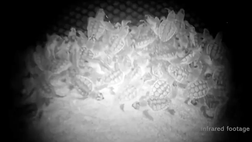
/https://tf-cmsv2-smithsonianmag-media.s3.amazonaws.com/filer_public/70/b4/70b4f1dc-f297-4e76-a1f4-b34438e53b27/gettyimages-2151346810_web.jpg)
/https://tf-cmsv2-smithsonianmag-media.s3.amazonaws.com/filer_public/58/42/58424895-992e-468d-9f24-32ac1b8d2028/gettyimages-945321410_web.jpg)
/https://tf-cmsv2-smithsonianmag-media.s3.amazonaws.com/filer_public/5a/d7/5ad75c46-898d-483f-a66e-1d05da661635/gettyimages-539707505_web.jpg)

:focal(800x602:801x603)/https://tf-cmsv2-smithsonianmag-media.s3.amazonaws.com/filer_public/0e/28/0e28f9dd-3e1e-49ef-b8ca-312becf2c959/1e0657_web.jpg)
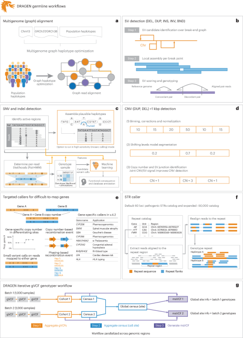


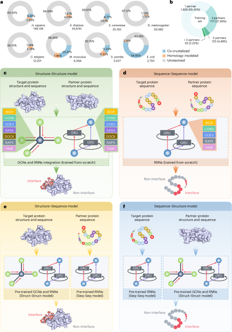
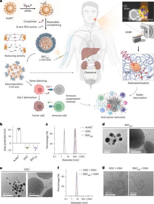

/https://tf-cmsv2-smithsonianmag-media.s3.amazonaws.com/filer_public/84/04/84049fd8-9f13-4b6f-8745-1ed7f3bfb329/animal1.jpg)
/https://tf-cmsv2-smithsonianmag-media.s3.amazonaws.com/filer_public/de/df/dedf95cf-1bf7-4499-9995-9710f8433be6/animal2.jpg)
/https://tf-cmsv2-smithsonianmag-media.s3.amazonaws.com/filer_public/87/09/8709e96f-4858-4418-83cf-3ce59481d36a/animal3.jpg)


/https://tf-cmsv2-smithsonianmag-media.s3.amazonaws.com/accounts/headshot/kim.png)
/https://tf-cmsv2-smithsonianmag-media.s3.amazonaws.com/filer_public/87/eb/87eb04bf-9885-4fde-a8cf-1a56cb914db5/1_pia21965_web.jpg)
/https://tf-cmsv2-smithsonianmag-media.s3.amazonaws.com/filer_public/1a/20/1a20b117-35a9-4759-b135-e230095bc23d/2_plutos_heart_-_like_a_cosmic_lava_lamp.jpg)
/https://tf-cmsv2-smithsonianmag-media.s3.amazonaws.com/filer_public/a2/27/a2275cbc-9402-4437-ad43-64cf6250e801/3_pia21590.webp)
/https://tf-cmsv2-smithsonianmag-media.s3.amazonaws.com/filer_public/58/b9/58b93f26-fd93-49e7-9b3e-2034c1c4194e/4_nh-pluto_cropjpg.webp)
/https://tf-cmsv2-smithsonianmag-media.s3.amazonaws.com/filer_public/d4/b5/d4b592f6-d403-4055-a259-2a0729d03559/5_top10_4plutovolcano.webp)
/https://tf-cmsv2-smithsonianmag-media.s3.amazonaws.com/filer_public/52/e0/52e0cbdb-23d5-4a49-bd37-bab395ac11dc/6_top10_10charon.webp)
/https://tf-cmsv2-smithsonianmag-media.s3.amazonaws.com/filer_public/59/7e/597e86ea-e568-4271-a50c-96a103518ae3/7_keane-pluto-wedge-annotated_web.jpg)
/https://tf-cmsv2-smithsonianmag-media.s3.amazonaws.com/accounts/headshot/alex.png)