Author: ANotiCiasabi

Optical setup and data acquisition

The Multi-SIM system was built on the basis of an invented fluorescence microscope (Ti2E, Nikon). Briefly, three laser beams of 488 nm (Genesis-MXSLM, Coherent), 560 nm (2RU-VFL-P-500-560, MPB Communications) and 640 nm (LBX-640-500, Oxxius) were combined collinearly and then passed through an acousto-optic tunable filter (AOTF, AOTFnC400.650, AA Quanta Tech). Afterward, the selected laser light was expanded and sent into an illumination modulator, which was composed of a ferroelectric spatial light modulator (SLM, QXGA-3DM, Forth Dimension Display), a polarization beam splitter and an achromatic half-wave plate. Different illumination modes were generated by adjusting the patterns displayed on the SLM, for example, grating patterns of 3 phases × 3 orientations at 1.41 numerical aperture (NA) for TIRF-SIM or 1.35 NA for GI-SIM. Next, the modulated light was passed through a polarization rotator consisting of a liquid crystal cell (Meadowlark, LRC-200) and a quarter-wave plate, which rotated the linear polarization to maintain the necessary S-polarization, thus maximizing the pattern contrast for all pattern orientations. The diffraction orders, except for ±1 orders for TIRF/GI-SIM, were filtered out by a spatial mask and then relayed onto the back focal plane of the objectives (1.49 NA, Nikon). The raw SIM images excited by different illumination patterns were sequentially collected by the same objective, then separated by a dichroic beam splitter (Chroma, ZT405/488/560/ 647tpc) and finally captured with an scientific complementary metal–oxide–semiconductor camera (Hamamatsu, Orca Flash 4.0 v3). We separately optimized the illumination pattern for each color channel and SIM reconstruction algorithm according to the objective NA and corresponding excitation wavelength, resulting in superior imaging quality for all channels in multicolor imaging. The Multi-SIM system integrates diverse imaging modes (TIRF/GI, TIRF/GI-SIM, three-dimensional (3D)-SIM, stacked slice-SIM, etc.) into a single setup, which is commercially available from NanoInsights.

In the BioTISR dataset, for each type of specimen and each imaging modality, we acquired the raw data from at least 50 distinct regions of interest (ROIs). For each ROI, we acquired 2–4 groups of raw images with N phases × M orientations × T time points with a constant exposure time but escalating excitation light intensity, where (N, M, T) corresponded to (3, 3, 20) for TIRF-SIM and GI-SIM, (5, 5, 10) for nonlinear SIM and (3, 5, 10) for 3D-SIM. Each set of N × M × T raw images were averaged as diffraction-limited time-lapse WF images or stacks, which were then used as the input LR image for TISR networks. Meanwhile, the raw images acquired with the highest excitation power were reconstructed into GT-SIM images or stacks, which served as the targets in model training. For better clarity, we summarize the imaging conditions and detailed information of the BioTISR dataset in Supplementary Table 1.

In long-term live-cell imaging experiments, cells were held in a stage-top incubator equipped on the microscope (OkO Lab, H301) to maintain conditions at 37 °C with 5% CO₂. We used the TIRF/GI mode and GI-SIM mode to acquire the WF or raw SIM images (which could be reconstructed into conventional SR-SIM images for comparison) and then obtained SR images using the DPA-TISR or Bayesian DPA-TISR models. The detailed imaging conditions of live-cell imaging experiments are summarized in Supplementary Table 2.

Network configurations for TISR model evaluation

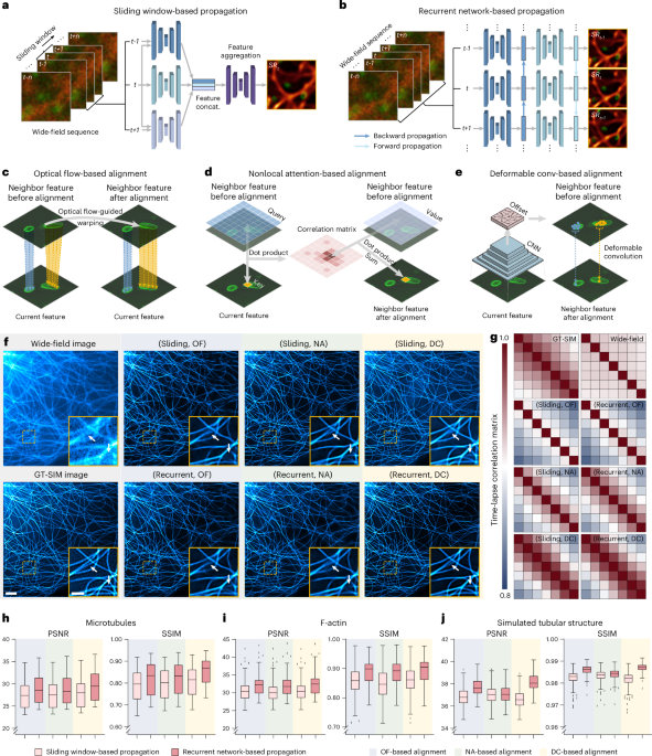
For fair comparison, we designed a template TISR model with the propagation and alignment modules replaceable, as depicted in Extended Data Fig. 2. The template TISR model was modified from the foundational BasicVSR++ neural network²¹. It comprises three primary modules: a feature extraction module, a propagation and alignment module and a reconstruction module. This architecture is meticulously crafted to be compatible with distinct components of the computational process. For a given image sequence X = {x_i−k, x_i−k+1, …, x_i, …, x_i+k−1, x_i+k}, three identical residual blocks are used to extract features from each frame. Each residual block comprises two convolutional layers, a leaky rectified linear unit activation function and a skip connection. Before passing through the residual blocks, a convolutional layer is applied for channel augmentation. The operation of feature extraction module can be formulated as

where f(∙) is a convolutional layer and RB is a residual block.

Subsequently, the output feature maps are fed into the propagation and alignment module through two distinct schemes, referred to as SWP and RNP.

In the SWP scheme, feature maps from the central and adjacent frames within a local window are severally fed into an alignment block to refine all neighbor features towards the central frame. The alignment block consists of an alignment module, a convolutional layer and three residual blocks. In our validation, three distinct alignment modules based on OF, DC and NA are used (Extended Data Fig. 2c–e). Afterward, the resulting feature maps are concatenated and go through a 1 × 1 convolutional layer to reduce the channels. The progress of SWP can be articulated as follows:

where \(\oplus\) denotes channel-wise concatenation and AB is an alignment block.

In the RNP scheme, the feature maps from adjacent frames generated by the feature extraction module propagate forward and backward in the time dimension following the second-order grid propagation manner²¹. Given the feature map \({x}_{i}^{1}\) and corresponding features propagated from the first-order neighborhood (h_i+1,h_i−1) and second-order neighborhood (h_i+2,h_i−2), we have

where \({g}_{i}^{\,\rm{backward}}\) and \({g}_{i}^{\rm{forward}}\) represent the feature computed at the ith timestep in backward and forward propagation, respectively.

In the OF-based alignment block, we compute the OF between neighbor frames using SPyNet⁴⁶. If we denote the OF from \({x}_{i-k}\) to x_i as \({f}_{i-k\to i}\), the neighbor features \({h}_{i-k}\) will be aligned according to \({x}_{i}\) by directly warping using the OF computed from \({x}_{i-k}\) and x_i:

where W denotes the spatial warping operation.

In DC-based alignment block, the OF \({f}_{i-k\to i}\) is used to prealign the features. The aligned features are then concatenated with the current features \({x}_{i}^{1}\) and OF \({f}_{i-k\to i}\) to compute the DC offset \({o}_{i-k\to i}\) and modulation mask \({m}_{i-k\to i}\) with two sequential residual blocks:

where σ denotes the sigmoid activation function. A DC layer is then applied to the unwrapped feature \({h}_{i-k}\):

where D denotes a DC.

In NA-based alignment block, three fully connected layers are initially used to generate the embedded query, key and value:

where F denotes a fully connected layer. Then, the NA mechanism is applied for feature alignment:

where \({\rm{\otimes }}\) refers to dot product operation. In practice, the embedded features have half of the channels compared to the original feature and we adopt a neighborhood attention mechanism⁴⁷, which can be regarded as a more efficient implementation of NA in our experiments, achieving similar SR performance.

Lastly, the aligned hierarchical features undergo through the reconstruction module consisting of three residual blocks, a pixel shuffle layer and a concluding convolutional layer to generate the SR residuals, which are then added up with upsampled raw input images, yielding final TISR images. The operation of the reconstruction module can be formulated as follows:

Taking the final output of RM as \({\hat{y}}_{i}\) and the GT as y_i for the ith frame, the overall objective function can be formulated as

The trainable parameter numbers of TISR models constructed as described are listed as follows: 5.58 million (sliding, OF), 5.59 million (sliding, NA), 7.97 million (sliding, DC), 3.95 million (recurrent, OF), 3.71 million (recurrent, NA) and 5.40 million (recurrent, DC).

Network architecture of DPA-TISR

DPA-TISR was constructed on the basis of the optimal TISR baseline model (that is, adopting recurrent network for propagation and DC for alignment), following the evaluation conclusions in Fig. 1. In DPA, as depicted in Fig. 2a and Extended Data Fig. 4b, the phase-space alignment mechanism serves as a complementary module to spatial DC, synergistically improving the alignment between neighborhood feature maps \({h}_{i-k}\) and current feature maps h_i. Specifically, the DPA begins with the real-valued fast Fourier transform (denoted as FFT(∙), implemented with torch.fft.rfft) to extract the amplitude and phase of both \({h}_{i-k}\) and h_i:

where \({\rm{Angle}}(\bullet )\) and \({\rm{Abs}}(\bullet )\) represent the operation to obtain the element-wise angle and absolute value of the features. Then. the concatenation of phases from current and neighborhood feature maps further goes through a phase-space convolution module, containing one convolutional layer followed by two residual blocks and a skip connection:

An inverse real-valued FFT (denoted as iFFT(∙), implemented with torch.fft.irfft) is then used to reconstruct the space-domain feature maps from the obtained amplitude and phase components:

The phase-refined feature maps are then fed into the DC module as depicted in Extended Data Fig. 2 for subsequent spatial alignment. The overall architecture of DPA-TISR is illustrated in Extended Data Fig. 4.

To adapt DPA-TISR to SIM reconstruction and volumetric SR inference, we further modified it into DPA-TISR-SIM and 3D DPA-TISR, respectively. The primary modifications are depicted in Supplementary Fig. 12 and described in detail in Supplementary Note 5.

Assessment metric calculation

We performed image normalization for GT-SIM and TISR images following a commonly used procedure^5,11. Specifically, each GT-SIM image stack Y was normalized by dividing by the maximum value, then blurred by a 3 × 3 size Gaussian kernel with the s.d. = 0.4 (denoted as ρ(∙)) to mitigate the SIM reconstruction artifacts:

Before computing the assessment metrics (that is, PSNR and SSIM), a linear transformation was applied to each SR image stack H:

where \({\rm{\alpha }}\) and \({\rm{\beta }}\) were chosen by solving the convex optimization problem:

where \({{||}\bullet {||}}_{2}\) denotes L₂ normalization. The optimized \(\alpha\) and \(\beta\) result in an MSE-minimized linear transformation of \({{H}}\), effectively scaling and translating every pixel to match the dynamic range of the GT.

Three types of metrics were used for quantitatively evaluating the performance in output fidelity, resolution and temporal consistency. PSNR and SSIM were used to evaluate pixel-level similarity between the inferred SR images and GT-SIM images. Decorrelation analysis⁴⁸ was applied to quantify the image resolution. For temporal consistency assessment, a time-lapse Pearson’s correlation matrix was used to visualize the similarity between adjacent SR images \({\{{H}_{i}\}}_{i=1}^{n}\). The Pearson correlation between images x and y is calculated by

where μ and σ denote the mean value and s.d. of corresponding images, respectively, and E represents the arithmetic mean.

Comparison of DPA-TISR with other models

For the comparative analysis between TISR and SISR models in Figs. 2 and 4 and Extended Data Fig. 7, we modified the 3D DPA-TISR into its SISR counterpart by excluding all operations related to alignment and propagation while keeping other network components (that is, the feature extraction module, reconstruction module and residual blocks in the alignment module), identical to (3D) DPA-TISR. As such, the temporal feature aggregation capability of 3D DPA-TISR was dismissed, yielding a pure SISR manner. Considering that the above SISR modification may cause a reduction in trainable parameters (for example, ~7 million for DPA-TISR versus ~5.5 million for SISR), we further compared DPA-TISR to its SISR counterparts with parameter compensation by adding additional residual blocks into SISR models (Supplementary Fig. 18), which verifies that the superiority of DPA-TISR over SISR mainly comes from the use of temporal information, rather than gain of trainable parameters.

In the comparative analysis between DPA-TISR and other TISR models (that is, VRT and BasicVSR++), we used their publicly available implementations on GitHub^21,27. All networks were trained with the same dataset and configurations (initial learning rate, learning rate decay, batch size, etc.) for fair comparison. It is noteworthy that the patch size of VRT was adjusted to 64, half that for other models, to ensure similar graphics processing unit (GPU) memory usage.

Implementation details of TISR models

The implementation procedure of TISR model typically includes three steps: training data preparation, model training and model inference. In this work, all TISR models were trained using the BioTISR dataset (Supplementary Table 1) unless otherwise stated. As described above, there are over 50 groups of paired WF–GT sequences for each biological specimen. Typically, we selected 40 of these groups for training and validation and used the remaining ~10 groups for testing. Before training, each group of data was augmented into time-lapse image pairs with the size of 128 × 128 × 7 for WF input and 256 × 256 × 7 or 384 × 384 × 7 for corresponding GT-SIM images by random cropping, horizontal or vertical flipping and random rotation for further enrichment and avoiding overfitting. In particular, we conducted an evaluation on DPA-TISR models trained with different lengths of input sequence and found that the input length of 7 was optimal to balance the computation efficiency and SR performance (Supplementary Fig. 19). In the live-cell experiments, we independently trained a specified DPA-TISR model for each type of biological structures (that is, each color channel) for best SR performance.

The training and inference were performed on a computer workstation equipped with four GeForce RTX 3090 graphic processing cards (NVIDIA) with Python 3.6 and PyTorch 1.12.1. In the model training procedure, the batch size for all experiments was set to 3 and all models were trained using the Adam optimizer with an initial learning rate of \(5\times {10}^{-5}\), which was decayed by 0.5 for every 1,000 epochs. The training process typically took 18 h within approximately 3,000 epochs. Once the networks were trained, TISR models could be applied to process other images of the same specimen, typically taking about 1 s to reconstruct a seven-frame SR stack of 1,024 × 1,024 pixels. The time required for both training and inference decreases linearly with the increase in the number of GPUs used and multi-GPU acceleration has been incorporated into our publicly available Python codes. Detailed instructions about environment installation, inference with pretrained model, training new models, confidence correction fine-tuning, etc. can be found in the GitHub repository of Bayesian DPA-TISR (https://github.com/liushuran2/Bayesian_DPA_TISR).

Calculation of uncertainty

The reliability of DPA-TISR predictions can be quantified through two types of uncertainties: model uncertainty and data uncertainty, also referred to as epistemic uncertainty and aleatoric uncertainty, respectively, in Bayesian analysis¹⁶.

Considering the non-Bayesian DPA-TISR, represented by \({f}_{\theta }\), where \(\theta\) indicates the trainable parameters, the output SR image sequence is denoted as \(\hat{{\rm{y}}}={f}_{\theta }(x)\). The network parameters are chosen by minimizing the pixel-wise distance between GT y and \(\hat{{\rm{y}}}\). Taking the L₁ loss as an example, the objective function can be expressed as follows:

where T denotes the number of time points and N denotes the number of pixels in a single image.

Inspired by previous work^11,17, we designed the Bayesian DPA-TISR that predicts both the intensity \({\hat{y}}_{n}\) and the scale \({\hat{\sigma }}_{n}\) for every pixel. Instead of considering each pixel as a single intensity value, we modeled it as a Laplace distribution empirically:

In this way, the scale \(\hat{\sigma }\) can be regarded as a measurement of the data uncertainty. Then, the output SR image \(\hat{y}\) and the scale \(\hat{\sigma }\) can be simultaneously addressed by minimizing the negative log-likelihood (NLL) function:

To characterize the model uncertainty, we adopted a Bayesian approximation approach¹⁷ that uses a distribution over model parameters by incorporating concrete dropout after convolutional layers. Within each inference, the dropout layers in Bayesian DPA-TISR randomly zeroized half of the neurons, thus yielding a distinctive model. Then, by aggregating a certain number (denoted as M) of the outcomes of the stochastic forward propagation, the SR results of Bayesian DPA-TISR can be obtained by averaging the predicted intensity of each trial:

where \({\hat{{{y}}}}^{(m)}\) is the predicted intensity map from the \({m}{\rm{th}}\) network. The model uncertainty is then quantified by calculating the standard deviation of the predicted results:

Subsequently, the overall data uncertainty is assessed as follows:

where \({\hat{\sigma }}^{(m)}\) is the predicted scale map from the \({m}{\rm{th}}\) network.

Calculation of confidence map

To enhance the integration of model and data uncertainty information and provide biologists with a more intuitive measurement of uncertainty, we take one step further by using a pixel-wise mixture probability distribution to generate an integrated confidence map.

During the inference stage, we independently generated M models \({\theta }^{(m)}\), differing only through dropout layers as depicted above. Considering inferences from M independent models, each pixel \(i\) follows a mixed Laplace distribution (example in Fig. 4a):

where \(\varOmega ={\{{\theta }^{(m)}\}}_{m=1}^{M}\) and \({x}_{p}\) is the coordinate of the PDF.

Accordingly, we defined the credible interval \({A}^{\varepsilon }=[{\hat{y}}_{\rm{mean}}-\varepsilon ,{\hat{y}}_{\rm{mean}}+\varepsilon ]\) and the interval length ε. Then, the corresponding confidence p^ε,i for pixel \(i\) is defined as the probability that the true value y falls within A^ε:

After defining a proper value for \({{\varepsilon }}\) (Supplementary Note 7), which was empirically set to 0.04 by default in our experiments, a confidence map can be generated to indicate the probability that the true value falls within the predicted credible interval.

Implementation details of Bayesian DPA-TISR

On the basis of the uncertainty and confidence calculation mentioned above, we designed Bayesian DPA-TISR, which differs from DPA-TISR in three main aspects. First, we integrated a dropout layer after each convolutional layer in the feature extraction module and reconstruction module, randomly deactivating neurons during both training and prediction stages. Notably, we did not apply dropout in the propagation and alignment module as we empirically found that any dropout here resulted in noticeable SR performance decline speculatively because of the temporal information loss during propagation and alignment (Supplementary Fig. 14b), while appropriate dropout (that is, with dropout rate lower than 0.5) in the feature extraction module and reconstruction module slightly benefited the overall SR performance (Supplementary Fig. 14c). Second, we adjusted the output channel number of the last convolutional layer in DPA-TISR from one to two, representing the predicted mean and scale, respectively. An additional sigmoid function was applied to the predicted scale channel to ensure its non-negativity. Third, the objective function was modified from L₁ loss to NLL loss as formulated in equation (24).

During inference stage, we independently executed the trained network with dropout six times (that is, M = 6), averaged the results as the final SR output and generated a confidence map as described previously. In particular, in long-term confidence-quantifiable TISR imaging experiments, we observed that the predicted scales tended to increase with the corresponding inferred intensities, making it unintuitive to discern which area of an output image is reliable or unreliable solely from the confidence map. To address this issue, we adopted an intensity-aware confidence generation scheme. Instead of using a constant \(\varepsilon\) of the credible interval \({A}^{\varepsilon }=[\,\hat{{{y}}}-\varepsilon ,\hat{{{y}}}+\varepsilon ]\) (hereafter, \({\hat{y}}_{\rm{mean}}\) is denoted by \(\hat{y}\) for simplicity), we modified the interval length \(\varepsilon\) as follows:

where the scalar scaling factor γ and ε were empirically set to 0.2 and 0.04, respectively, in our experiments. Using \(\bar{\varepsilon }\) essentially defines a threshold of 0.2 for foreground segmentation. For pixels with values greater than 0.2, which are more likely to belong to the actual structure, we assigned a proportion (0.2) of their absolute intensity as the interval length. Conversely, for pixels with values less than 0.2, typically representing the background region, we assigned a constant value of 0.04 as the interval length, thereby rationalizing the confidence calculation within background regions of the inferred TISR image.

Calculation of ECE and reliability diagram

To evaluate the effectiveness of the uncertainty and confidence map, the reliability diagram that compares the empirical accuracy to averaged confidence was computed following a standard procedure¹¹ in our experiments. Well-calibrated confidence in the reliability diagram should yield confidence values similar to accuracy, resulting in a diagonal diagram.

Specifically, the empirical accuracy is defined as the proportionality that the GT \(y\) falls into the credible interval \({A}^{\varepsilon }=[\,\hat{{{y}}}-\varepsilon ,\hat{{{y}}}+\varepsilon ]\). Consequently, the accuracy and confidence are specified as follows:

where \({{S}}\) denotes a subset of all pixels, 1(∙) denotes the indicator function and ε > 0 determines the length of the credible interval around each \(\hat{{{y}}}\).

To construct a reliability diagram with K groups, we divided the value of confidence into K intervals segmented by τ₀, τ₁, …, τ_K. For pixels in \({S}_{k}^{\varepsilon }=\{{p}^{\varepsilon }\epsilon ({\tau }_{k-1},{\tau }_{k}]\}\), we plotted \({\rm{Confidence}}(\,{{\hat{y}},{\hat{f}}\,{|}S}_{k}^{\varepsilon },{{\varepsilon }})\) against \({\rm{Accuracy}}(\,{{\hat{y}},{y\; |}S}_{k}^{\varepsilon },{{\varepsilon }})\) to obtain the final reliability diagram. Furthermore, the ECE was determined as the weighted average of the absolute differences between the accuracy and confidence:

Confidence correction for Bayesian DPA-TISR

Recognizing the disparity between the estimated confidence and actual accuracy (that is, overconfidence for most Bayesian neural networks), we developed an iterative fine-tuning framework to eliminate the ECE between the estimated confidence and accuracy. During the fine-tuning stage, the objective function was modified from equation (24) as follows:

where \({R}_{\rm{confidence}}\) is the CCR and \(\alpha\) is a weighting scalar to balance \({{\mathscr{L}}}_{{NLL}}\) and \({R}_{\rm{confidence}}\), which was empirically set to 0.1 in our experiments. CCR comprises two parts:

where the second term, \({\rm{confidence}}\left({\hat{y}},{\hat{f}}\,|{{\varepsilon }}\right)\), is the average confidence of the outputs and the corresponding weighting scalar \(k\) aims at adjusting overall average confidence of prediction. Positive values of k suppress overconfidence and negative values of k restrain underconfidence, which is the key variable in our optimization framework. We adopted a combined strategy of linear searching and parabola fitting to determine the optimal value of k.

In the optimization process, a relative ECE (rECE) of the original trained network, denoted as E₀, is first calculated by

of which the sign is used to determine the initial direction for subsequent optimization:

where \({\Delta}\) is the step size set to 0.1 by default. Next, the first two trials of fine-tuning are independently performed with \({k}_{1}\) and \({k}_{2}\), respectively, using the objective function described in equation (34), after which we obtain two new ECE values of the fine-tuned networks, denoted as \({E}_{1}\) and \({E}_{2}\). If \({E}_{1} < {E}_{2}\), we exchange \({k}_{1}\) and \({k}_{2}\), as well as the corresponding \({E}_{1}\) and \({E}_{2}\), and reverse the searching direction (that is, reset \({\Delta}\) as −0.1) to ensure that \({k}_{2}\) is the ECE-descent direction compared to \({k}_{1}\). Afterward, the linear searching process continues along this descent direction,

until finding a \({k}_{i}\) value that satisfies \({E}_{i} > {E}_{i-1}\), where \({E}_{i}\) denotes the ECE value of the fine-tuned model with \({k}_{i}\). We then use the quadratic polynomial fitting to find the optimal \({k}_{* }\) value according to the three latest weighting scalars \({k}_{i},\,{k}_{i-1},\,{k}_{i-2}\) and corresponding ECE values \({E}_{i},{{E}}_{i-1},\,{E}_{i-2}\):

One final fine-tuning is carried out using the optimal \({k}_{* }\) in the objective function to obtain a confidence-calibrated Bayesian DPA-TISR model. During the fine-tuning stage, the model was trained using the Adam optimizer with an initial learning rate of \(5\times {10}^{-5}\), which is decayed following a cosine annealing strategy over a course of 30 epochs. The overall fine-tuning process typically takes less than 1 h. The workflow diagram of the confidence correction is shown in Supplementary Fig. 20.

Mito–PO contact quantification

The contact level between Mito and POs was evaluated by confidence-weighted MOC. Considering that Mito–PO contact sites were principally situated at the periphery of POs, we first identified the boundary of each PO using the following procedure: (1) the background of the ROI of the PO was estimated by applying a Gaussian filter with s.d. = 10 pixels; (2) the TISR image was smoothed using another Gaussian filter with s.d. = 1 pixel and then the estimated background was subtracted; (3) a binary mask was generated by setting a threshold to the background-subtracted image; (4) the boundary of each PO was extracted using the Sobel operator; and (5) the PO boundary image was convolved with the equivalent PSF of SIM, thereby delineating potential contact regions of POs. Next, following steps 1–3, a binary Mito mask, denoted as \({{{M}}}_{{\rm{Mito}}}\), was calculated.

We reasoned that the regions with higher confidence should have higher weights in MOC calculation. Therefore, we applied the confidence map estimated by the Bayesian DPA-TISR model as adaptive wights to rationalize the quantification of Mito–PO contacts as follows:

where \({{{Y}}}_{{{i}}}\), \({{{M}}}_{{\rm{Mito}},{{i}}}\) and \({{{C}}}_{{\rm{Mito}},{{i}}}\) denote the value of the \({i}{\rm{th}}\) pixel in the ROIs of the PO boundary image \({{Y}}\), Mito mask \({{{M}}}_{{\rm{Mito}}}\) and the confidence map \({{{C}}}_{{\rm{Mito}}}\).

Cell culture, transfection and staining

COS-7 and HeLa cells, as well as their stable cell lines, were cultured in DMEM (Gibco, 11965092), supplemented with 10% FBS (Gibco, 10099141C) and 1× penicillin–streptomycin (Thermo Fisher Scientific, 15140122) at 37 °C in a Thermo Fisher Scientific Heracell 150i CO₂ incubator. SUM159 cells were cultured in DMEM/F12K medium supplementary with 5% FBS and 1% penicillin–streptomycin solution.

For live-cell imaging, the 35-mm coverslips were precoated with 50 μg ml⁻¹ collagen and 1 × 10⁵ cells were seeded onto coverslips. For transient transfection, cells were transfected with plasmids using Lipofectamine 3000 (Invitrogen, L3000150) according to the manufacturer’s protocol 12 h after plating. Cells were imaged for 12 h after transfection. Where indicated, the cells transfected with Halo-tagged plasmids were labeled with 10 nM JF549 ligand for 15 min according to the published protocol⁴⁹. The cells were rinsed with fresh medium to remove unbound ligand and imaged immediately afterward. The plasmids used in transient transfection included Lifeact–mEmerald, Lifeact–SkylanNS, Clathrin–mEmerald, Clathrin–mCherry, 3×mEmerald–Ensconsin, Lamp1–Halo, 2×mEmerald–Tomm20, TFAM–mEmerald, PKMO–Halo and PMP–Halo.

Statistics and reproducibility

Figures 1h–j and 2e,f and Extended Data Figs. 3c,d, 5f,h, 6c,d and 7e were plotted in Tukey box-and-whisker format. The box extends from the 25th and 75th percentiles and the line in the middle of the box indicates the median. The upper whisker represents the larger value between the largest data point and the 75th percentile plus 1.5× the interquartile range (IQR) and the lower whisker represents the smaller value between the smallest data point and the 25th percentile minus 1.5× the IQR. Data points larger than the upper whisker or smaller than the lower whisker were identified as outliers and are displayed as black spots.

Reporting summary

Further information on research design is available in the Nature Portfolio Reporting Summary linked to this article.

Setup of AAV capsid testing in human liver

We first investigated the possibility of long-term NMP with the commercially available OrganOx metra system²⁰ (beyond the 24 h used clinically) using a steatotic and fibrotic human liver (steatotic liver 1 (SL 1); Extended Data Fig. 1a–c and Supplementary Table 1). We replaced 20% of the perfusate with PRBCs every 24 h or when the hemoglobin dropped to 6 g dl^–1. We evaluated the perfused liver according to the same criteria used clinically for selecting transplantable livers by short-term NMP²¹. The liver was viable and functional for 103 h, as evidenced by lactate clearance (<2.5 mmol l^–1), glucose metabolism (responsiveness to insulin) and pH (7.3–7.4), all measured in the perfusate, and bile production (>4 ml h^–1; Extended Data Fig. 1d). In addition, the liver remained responsive to continuous infusion of a vasodilator by maintaining a stable hemodynamic profile (Extended Data Fig. 1e).

To optimize long-term NMP, we added basic renal function by incorporating a hemoconcentrator into the NMP circuit, which we tested in another steatotic liver (SL 2; Extended Data Figs. 1a and 2a). After 3 h of hemoconcentration, levels of blood urea nitrogen, creatinine and osmolality in the perfusate were reduced by about 20%, reflecting removal of waste metabolites (Extended Data Fig. 2b). We balanced electrolyte levels by replacing the hemofiltrate with isotonic dialysate (Extended Data Fig. 2c).

We also used perfusion of SL 2 to eliminate biases from our approach to AAV capsid evaluation. We removed residual plasma, which can include NAbs to AAV capsids^27,28, by centrifugation-mediated washing of PRBCs²⁹, after which NAbs to the AAV2, AAV5, AAV6, AAV8 and AAV-DJ capsids became nearly undetectable as assessed by luciferase-based neutralization assay (Extended Data Fig. 3a). We also excluded loss of AAV vectors by attachment to the surface of the silicone tubing in the NMP circuit³⁰ (Supplementary Fig. 1).

Finally, we minimized the time required to detect functional transduction, that is, mRNA and protein expression by AAV vectors. We constructed a self-complementary AAV (scAAV) vector that expresses a fluorescent protein-encoding transgene from the cytomegalovirus (CMV) promoter. scAAV vectors express transgenes more rapidly than single-stranded AAV vectors because they bypass the need for second-strand DNA synthesis after uncoating of the viral particle in the nucleus³¹. The CMV promoter is ubiquitously active, which allows for comprehensive characterization of AAV capsid tropism³². Moreover, the CMV promoter provides rapid-onset and high-level transgene expression—it is subject to silencing in hepatocytes but only after 7 days³³. To identify the earliest time point when functional transduction could be reliably detected, we intravenously injected scAAV vectors produced with AAV8, AAV5, AAV-LK03 and AAV6 capsids into mice. Expression of vector-derived mRNA and fluorescent protein increased moderately between 48 h and 7 days after injection, reflecting ongoing functional transduction, but the relative transduction efficiencies of the four AAV vectors were essentially the same between the two time points (Supplementary Fig. 2a,b). These results led us to use the scAAV-CMV vector for all subsequent experiments (Supplementary Table 2).

These results establish NMP as an experimental system for testing AAV capsids under physiological conditions in human livers and limit the critical perfusion time after AAV vector administration to 48 h.

Transduction profile of the AAV8 capsid in normal human liver

Using our optimized approach, we investigated the efficiency and specificity of hepatocyte transduction of a vector produced with the AAV8 capsid, which is most commonly used in clinical trials of liver gene therapy¹, in two human livers that were histologically normal according to biopsies taken before NMP (Supplementary Fig. 3 and Supplementary Table 1). Perfusate obtained before vector infusion contained a negligible amount of NAbs to the AAV8 capsid, confirming the efficacy of PRBC washing (Extended Data Fig. 3b). After achieving an optimal hemodynamic and metabolic profile at 12 h of perfusion, we infused 5.7 × 10¹² vector genomes (vgs) of AAV8–enhanced green fluorescent protein (AAV8–eGFP) into normal liver 1 (NL 1) and 1.6 × 10¹³ vgs of AAV8–enhanced yellow fluorescent protein (AAV8–eYFP) into NL 2 through the portal vein (Fig. 1a–c, Extended Data Fig. 4a and Supplementary Table 2). These doses reflect the range given in clinical trials of liver gene therapy with AAV8 vectors³ but are calculated based on liver weight instead of body weight because biodistribution is not a factor in our system (Supplementary Table 1). We ascertained the functionality of these AAV vectors after intravenous injection into mice (Extended Data Fig. 5a). Declining vector DNA levels in the perfusate indicated uptake into the liver (Supplementary Fig. 4a–c). We ended NMP when the lactate level began increasing to ascertain a physiological state (48 h after AAV infusion for NL 1 and 50 h for NL 2; Fig. 1c and Extended Data Fig. 4a).

After NMP ended, we enzymatically released hepatocytes and nonparenchymal cells (NPCs), including endothelial cells, monocytes/macrophages, cholangiocytes and mesenchymal cells (hepatic stellate cells and fibroblasts), and analyzed them by single-cell RNA sequencing (scRNA-seq). Analysis of 6,959 cells from NL 2 showed 6 principal and 14 specific cell types (Fig. 1d and Supplementary Fig. 5a–e), with hepatocytes being most efficiently transduced by the AAV8 vector, closely followed by endothelial cells and monocytes/macrophages (Fig. 1e). Immunostaining of fluorescent protein-expressing cells in tissue sections and flow cytometry with optimized antibody panels (Extended Data Fig. 6a–d) confirmed the AAV8 capsid tropism identified by scRNA-seq independent of vector dose (Fig. 1f,g). Quantitative digital droplet PCR (ddPCR) showed dose-dependent differences in vector DNA and transgene mRNA in isolated hepatocytes and tissue samples of the eight liver segments from the two livers, with tight correlation between the two parameters (Fig. 1h,i). In situ hybridization (ISH) with sense or antisense probes targeting vector DNA or both vector DNA and transgene mRNA confirmed this result (Fig. 1j).

These results show that the tropism of the AAV8 capsid in the normal human liver includes endothelial cells and monocytes/macrophages in addition to hepatocytes. These results also establish that the AAV8 capsid affords efficient functional transduction in the human liver as evidenced by corresponding levels of physical vector cell entry and transgene expression, with scRNA-seq being equally as informative as flow cytometry.

Comparison of AAV capsids in normal and steatotic human livers

We compared the transduction profile of the AAV8 capsid with that of the AAV5, AAV-LK03 and AAV6 capsids, which are most commonly used in clinical trials of liver gene therapy¹, and the AAV-NP59 capsid, which, based on studies in immune-deficient mice, has the strongest tropism for human hepatocytes³⁴. To facilitate side-by-side comparison, for each capsid, we introduced a unique fluorescent protein-encoding transgene and expressed barcode into the AAV vector, allowing for distinction by flow cytometry, microscopy and ddPCR (Supplementary Fig. 6a–d and Supplementary Table 2). We ascertained that scRNA-seq reliably detects transgenes and barcodes (see Methods) and excluded that co-injection of AAV vectors produced with the different capsids alters the transduction efficiency of any individual capsid in mice (Supplementary Fig. 6e,f).

Before testing in human liver, we intravenously co-injected the AAV vectors at the same dose into wild-type mice and FRGN mice repopulated with human hepatocytes. Two days later, we enzymatically released hepatocytes and analyzed fluorescent protein expression by flow cytometry. We found a capsid-specific transduction efficiency of AAV8 > AAV6 > AAV5 > AAV-LK03 > AAV-NP59 in mouse hepatocytes and AAV-NP59 > AAV-LK03 > AAV8 > AAV6 > AAV5 in human hepatocytes (Extended Data Fig. 5b–h), which is in agreement with reports of species-specific hepatocyte tropism of these capsids^{10,11,12,13,34}.

Because the anticoagulant heparin used for NMP in the clinical setting can reduce the transduction efficiency of the AAV-LK03, AAV6 and AAV-NP59 capsids^35,36, we substituted low-molecular-weight heparin after screening alternative anticoagulants in mice (Supplementary Fig. 7a–c).

We co-infused AAV vectors produced with the five capsids into four human livers, two histologically normal (NL 3 and NL 4) and two steatotic (SL 3 and SL 4; Supplementary Fig. 3 and Supplementary Table 1). To contextualize our results, we sequentially introduced additional AAV vectors in combination with AAV8, which served as an internal control, with the AAV8, AAV5, AAV-LK03, AAV6 and AAV-NP59 capsids being tested in four, four, three, one and one livers, respectively (Fig. 2a). We co-infused AAV vectors at the same dose, ranging from 6.7 × 10¹¹ vgs to 3.4 × 10¹³ vgs per vector between livers (Supplementary Table 2). Both normal and steatotic livers were viable, as assessed by analysis of liver injury and function in perfusate and cell death in tissue sections, and hemodynamically stable throughout NMP, up to and including the termination time of 60–73 h after AAV vector infusion (Extended Data Fig. 4a,b). We retrieved hepatocytes and NPCs at high yield from all livers, allowing for integrated clustering of 6 principal and 26 specific cell types by scRNA-seq (Fig. 2b and Supplementary Fig. 8a). All five AAV vectors primarily transduced hepatocytes. Among NPCs, endothelial cells and myeloid cells were most frequently transduced, whereas cholangiocytes, mesenchymal cells and lymphocytes showed low levels of transduction (Fig. 2c,d). Notably, AAV-LK03 was most specific for hepatocytes, with minimal transduction occurring in NPCs.

We next quantified capsid-specific transduction at the mRNA, protein and DNA levels in hepatocytes by scRNA-seq, flow cytometry and ddPCR. In hepatocytes, we found a functional transduction (mRNA and protein) efficiency of AAV-LK03 > AAV-NP59 > AAV8 ≥ AAV6 > AAV5 (mRNA range: 27.7% to 0.3%, protein range: 23% to 0.3%) and a physical transduction (DNA) efficiency of AAV6 > AAV-NP59 > AAV-LK03 > AAV8 > AAV5 (range: 70.9 to 2.2 vgs per diploid genome; Fig. 2e–i and Supplementary Fig. 9a–d). The relative transduction efficiency in the eight segments of each liver paralleled the levels in hepatocytes, which we confirmed in tissue sections by ISH of vector DNA and mRNA (Supplementary Figs. 10a–c and 11a–d). Detection of unique capsid barcode sequences alone by scRNA-seq further confirmed the capsid transduction hierarchy (Supplementary Fig. 10d). Notably, the functional transduction efficiency of AAV-NP59 was 55% less than that of AAV-LK03, the opposite of what has been reported in immune-deficient mice engrafted with human hepatocytes, which we independently confirmed³⁴ (Extended Data Fig. 5e,f,h).

We also investigated capsid-specific differences in transcription efficiency by quantifying the ratio of AAV transgene mRNA to uncoated AAV vgs within nuclei, that is, DNA available for transcription (Supplementary Fig. 10e–g). Transcription efficiency was highest for AAV-LK03 and lowest for AAV5 (Fig. 2j).

These results show that the AAV-LK03 capsid transduces hepatocytes in human liver much more efficiently and specifically than the AAV-NP59, AAV8, AAV6 and AAV5 capsids. By establishing the superiority of AAV-LK03 for hepatocyte-targeted human liver gene therapy, our results highlight limitations of immune-deficient mice engrafted with human hepatocytes³⁴. In addition, these results uncover capsid-specific effects on AAV vector transcription in the human liver, which aligns with reports of an epigenetic role of the AAV capsid^37,38.

AAV capsid-specific effects of hepatocyte zonation and steatosis

To determine whether any of the five AAV capsids preferentially transduces hepatocytes in a specific zone of the human liver and how this tropism may be altered in the setting of steatosis, we analyzed scRNA-seq data from 22,146 hepatocytes from NL 3, NL 4, SL 3 and SL 4. We generated a periportal and pericentral score derived from the expression of zonation markers conserved across all four livers to quantify the zonation enrichment on a per cell basis (Extended Data Table 1), which revealed a consistent pattern of functional zonation irrespective of disease state (Fig. 3a and Extended Data Fig. 7a). Similarly, in assessing the effect of steatosis on these parameters, we adopted a nonbinary approach to cell classification by scoring each cell individually based on expression of steatotic marker genes (Fig. 3a and Extended Data Table 1). This approach revealed a spectrum of steatosis, with normal livers containing some steatotic cells and steatotic livers containing some normal cells, and enabled us to identify CXCL8 as a highly specific and conserved marker of steatotic hepatocytes across normal and steatotic livers (Extended Data Table 1 and Extended Data Fig. 7b).

We also investigated whether the most steatotic hepatocytes exhibit altered transcriptomic signatures. We focused on hepatocytes from SL 4, the most steatotic liver by histologic score, because 42% of these hepatocytes clustered separately from the other livers despite integration (Extended Data Fig. 7c). These clusters were uniquely enriched for expression of genes in the NADPH reduction pathway (TXNRD1, GCLM, AKR1C1 and AKR1C2), which plays an important role in fatty acid biosynthesis³⁹ (Extended Data Fig. 7d,e). Zonation was retained in these cells, consistent with it being altered only in end-stage liver disease⁴⁰ (Fig. 3a and Extended Data Fig. 7a).

These results showed that our steatosis scoring method accurately reflects tissue histology and that our zonation scoring method is applicable to all livers regardless of steatosis severity. We applied these methods to determine the effects of steatosis on AAV capsid transduction at single-cell resolution. We first compared AAV capsid behavior by plotting hepatocytes transduced with the three capsids most commonly used in clinical trials against their respective zonation and steatosis scores (Methods and Fig. 3b). This analysis revealed higher periportal scores for AAV8 and AAV-LK03 than for AAV5, which conversely showed unique pericentral score enrichment. AAV5 transduction was associated with a higher steatosis score, which reflected its high pericentral score⁴¹ (Fig. 3b).

Next, we analyzed normal and steatotic livers separately to determine the contribution of disease state to zonation of AAV capsid transduction. Our scoring method showed that the weak periportal zonation of AAV8 was specific to normal livers (Fig. 3c), whereas pericentral zonation of AAV5 was specific to steatotic livers (Fig. 3d), which we confirmed in tissue sections by ISH of vector DNA (Fig. 3e) and/or mRNA (Supplementary Fig. 11a–d). We found differential expression of genes associated with steatosis and steatotic liver disease in hepatocytes exclusively transduced by AAV5. Pericentrally zonated LPCAT2 (ref. ⁴²) and LPCAT1, genes involved in phosphatidylcholine biosynthesis and lipid droplet formation and remodeling⁴³, were enriched, whereas FADS1, which protects hepatocytes from lipid accumulation⁴⁴, and FADS2 were depleted in SL 3; C3AR1 and DUSP9, which regulate lipid accumulation^45,46, were enriched in SL 4, and pericentrally zonated SLCO1B3 (ref. ⁴⁷) was enriched in both steatotic livers (Supplementary Data 1). ISH confirmed that AAV5 favors steatotic pericentral hepatocytes by showing vector DNA (Fig. 3e) and/or mRNA (Supplementary Fig. 11a,d) accumulating in lipid-laden cells. There were also steatosis-dependent changes in AAV-LK03 zonation. The strong periportal zonation of AAV-LK03 observed in normal liver was lost in the setting of steatosis, where its pericentral zonation was increased, which we confirmed by ISH of tissue sections (Fig. 3f,g and Supplementary Fig. 11b–d). For AAV6, our zonation model and ISH showed weak periportal zonation in normal liver, whereas AAV-NP59 showed pericentral zonation in steatotic liver (Extended Data Fig. 7f and Supplementary Fig. 11c,d). These tropisms could not be explained by the presence or absence of known AAV entry factors⁴⁸ (Supplementary Fig. 8b,c). A high steatosis score did not negatively impact the transduction efficiency of any of the AAV capsids we tested (Fig. 3c,d,f).

Notably, we identified a population of nonzonated hepatocytes both in normal and steatotic livers marked by the expression of SOX9, SPP1 and TACSTD2 (Extended Data Fig. 7g–i). The number of TACSTD2 (TROP2)-expressing hepatocytes increased considerably with steatosis severity, which was not paralleled by an increase in markers of proliferation (Extended Data Fig. 7j,k), suggesting that TROP2 expression in hepatocytes reflects reaction to disease, not expansion of a progenitor cell population as previously suggested¹⁹. The cells can be transduced by all capsids we tested, with AAV-LK03 being the most efficient, which highlights this hepatocyte population as a potential therapeutic target in steatotic liver disease (Extended Data Fig. 7l).

These results show that the AAV-LK03 capsid preferentially transduces periportal hepatocytes in normal human liver but lacks this zone-specific tropism in the steatotic human liver. AAV8 shows similar trends, but its periportal hepatocyte tropism is much less pronounced in human liver than in NHP liver¹⁶. Meanwhile, the AAV5 capsid has a strong tropism for pericentral hepatocytes in the steatotic human liver but transduces hepatocytes evenly in the normal human liver⁴⁹.

AAV capsid-specific and steatosis effects on vector episome formation

We next investigated whether steatosis impacts episome formation of AAV vectors, which is critical for long-term transgene expression⁵⁰. We isolated nuclei from liver tissue from NL 2, NL 3, NL 4, SL 3 and SL 4 to quantify vector episomes using digital PCR (Fig. 4a and Methods)⁴⁹ and confirmed that circular monomers and concatemers form in human livers within 73 h (Fig. 4b,c). We found fewer vgs in episomes isolated from steatotic livers than in episomes isolated from normal livers, independent of which of the five AAV capsids was used to produce the vector, suggesting that circular concatemerization of AAV vectors was compromised in steatotic livers (Fig. 4d).

To confirm this result, we analyzed episome formation by vectors produced with the AAV8, AAV5 and AAV-LK03 capsids cotransduced into human induced pluripotent stem cell-derived hepatocytes (iPS cell-Heps) treated with palmitic acid, a saturated fatty acid that causes steatosis⁵¹. As a prerequisite, we ascertained that cotransduction does not impact quantification of episome formation (Extended Data Fig. 8a–c). We found that palmitic acid treatment for 7 days caused the number of episomes to decline (Fig. 4e,f). Palmitic acid had little effect on physical transduction and transgene expression, indicating that not only episomes but also linear vectors are available for transcription soon after transduction (Extended Data Fig. 8d,e). Confirming our findings in human livers, AAV8 and AAV-LK03 vectors failed to form concatemers in steatotic iPS cell-Heps, whereas the AAV5 vector was unaffected because it predominantly formed circular monomers despite a high number of transduced vgs (Fig. 4g and Extended Data Fig. 8d).

Next, we investigated long-term episome formation by AAV vectors, focusing on the distinctive effect of the AAV5 capsid, leading to predominant formation of circular monomers in human livers (Fig. 4b–d and Extended Data Fig. 8f). We analyzed AAV8, AAV5 and AAV-LK03 episomes in FRGN mice repopulated with human hepatocytes to more than 90% (ref. ⁵²). The number of vgs in AAV8 and AAV-LK03 episomes was stable for 70 days, and they rapidly formed large concatemers (Fig. 4h–j). This finding confirms findings in livers of NHPs where concatemers formed as early as 3 days and lasted for 90 days after intravenous injection of an AAV8 vector⁵³. By contrast, the number of vgs in AAV5 episomes declined over time, probably because of degradation, with concatemers being detectable only by day 42. The number of vgs in episomes dictated the transcriptional output at all time points for all capsids, with linear vgs probably contributing to transcription initially (Extended Data Fig. 8g,h). AAV5 episomes had the lowest transcription efficiency across all time points, contradicting previous findings in mouse liver that monomers are more efficiently transcribed than concatemers⁵⁴. Episome kinetics of these capsids were similar in wild-type mice, with AAV5 showing rapid circular monomer formation followed by a steep decline in the number of vgs in episomes and concatemerization occurring only by day 40 (Extended Data Fig. 8i–l).

These results reveal that the AAV capsid influences the kinetics of vector episome formation, probably by affecting the recombination of inverted terminal repeats (ITRs)⁵⁵. The AAV5 capsid causes formation of relatively unstable episomes that concatemerize more slowly than AAV8 and AAV-LK03 episomes, which translates into lower long-term transgene expression. In addition, these results identify steatosis as a capsid-independent factor impairing episome concatemerization and thereby the durability of transgene expression from AAV vectors.

AAV capsid-specific nonhepatocyte tropism and co-regulated genes

The tropism of AAV capsids for human liver cell types beyond hepatocytes is unknown, which may have contributed to complications or obscured opportunities in the clinical setting. Our integrated dataset from NL 3, NL 4, SL 3 and SL 4, including over 35,800 cells and 26 specific cell types, revealed that AAV vectors consistently transduce not only hepatocytes but also endothelial cells and monocytes/macrophages (Fig. 2c,d). We separately analyzed all endothelial cells and monocytes/macrophages to identify potential heterogeneity in transduction within these populations. From 2,759 monocytes/macrophages, we discerned seven distinct types, including scar-associated macrophages reported in fibrotic livers⁵⁶ that were most prevalent in SL 3 and SL 4 (Fig. 5a,b and Extended Data Fig. 9a). We found a clear tropism for resident Kupffer cells of all capsids except AAV-LK03, with AAV6 and AAV8 being most efficient, transducing up to 13.2% and 8.6% of Kupffer cells, respectively (Fig. 5b–e).

Subclustering of 2,091 endothelial cells distinguished eight subpopulations, of which the five capsids almost exclusively transduced liver sinusoidal endothelial cells (LSECs), with AAV5 and AAV8 being most efficient (Fig. 5f–j and Extended Data Fig. 9b). In steatotic livers, AAV5 transduced LSECs 3.3–5 times better than AAV8 to a maximum of 3.5%, whereas in normal livers, AAV8 was equivalent or better than AAV5 at 2% (Fig. 5j and Extended Data Fig. 9c). This unique tropism probably reflects the increase in immune-polarized LSECs in steatotic livers, which were transduced more readily by AAV5 (Fig. 5g,i). These results indicated that, as with hepatocytes, the steatotic environment increases the transduction of LSECs by AAV5. In addition, these results highlighted LSECs (the physiological source of factor VIII and von Willebrand factor) as an alternative and more physiologically relevant target than hepatocytes for hemophilia A⁵⁷ or von Willebrand disease gene therapy^58,59. In support of this notion, the transduction efficiency of LSEC subtypes by the AAV8 and AAV5 capsids approached or surpassed levels found in hepatocytes transduced with the same capsids (Figs. 2d and 5i). Moreover, 1.25% of total LSECs expressed MKI67 or TOP2A, which is comparable to the 1.30% of hepatocytes found to express these markers and suggests a similar turnover rate and thus AAV vector persistence between the two cell types⁶⁰ (Extended Data Fig. 9d).

Finally, we sought to define potential host factors involved in or affected by transduction of the five AAV capsids in hepatocytes from NL 3, NL 4, SL 3 and SL 4 (Supplementary Data 1). We found no evidence for activation of inflammatory signaling by AAV vectors in hepatocytes (Supplementary Fig. 8d). Differential gene expression analysis of 3,749 hepatocytes uniquely transduced with one of the five AAV vectors further showed that most upregulated genes exhibit a modest increase in expression (log₂ (fold change) < 1), indicating that AAV vectors do not perturb the host cell transcriptome (Supplementary Data 1). Focusing on significantly coenriched genes common to at least three capsids highlighted PIGR, which regulates the transcytosis of immune complexes for defending against viral infection⁶¹, and APOC1, a cofactor mediating hepatitis C virus infection⁶². CSH2 was the most significantly coenriched gene in hepatocytes transduced with the AAV8, AAV-LK03 or AAV-NP59 capsid in NL 2, NL 3 and SL 4 (Supplementary Data 1 and Supplementary Fig. 12a,b). Despite evidence that CSH2 plays a role in regulating hepatitis B virus transcription⁶³ or in the virus defense response⁶⁴, its role in AAV vector transduction is unknown.

These results define the human NPC tropism of the four AAV capsids most commonly used in clinical trials of liver gene therapy¹ and a promising new capsid engineered to specifically transduce human hepatocytes³⁴. Illustrating the value of these results, they suggest LSECs as a physiological target for gene therapy of hemophilia A or von Willebrand disease using the AAV5 or AAV8 capsid. These results also highlight capsid-specific genes potentially involved in AAV trafficking or transcription and show transcriptomic stability of hepatocytes transduced with AAV vectors.

Nota do editor A natureza de Springer permanece neutra em relação às reivindicações jurisdicionais em mapas publicados e afiliações institucionais.

Este é um resumo de: Schuhknecht, L. et al. Um mapa metabólico humano de perturbações farmacológicas revela modos de ação medicamentosos. Nat. Biotechnol. https://doi.org/10.1038/S41587-024-02524-5 (2025).

What do nine Hawaiian snails have in common with the Texas longhorn, the Florida panther and the California grizzly bear? They’re all U.S. state animals. And the snails hold another notable distinction—they are the country’s first-ever state gastropods.

This past April, Hawaii enacted a law to designate nine species of kāhuli—the Hawaiian word for the native land snails—as the state’s official snails. At an event held for the signing of the bill into law at the governor’s residence, jarred specimens of the nine kāhuli decorated a table. Before committing his pen to paper, Governor Josh Green told lawmakers, students and malacologists—scientists who study mollusks, including snails—that the legislation passed as a direct result of their advocacy.

But the story of Hawaii’s state snails originated with one student, who created a movement that gained momentum long after they graduated, inspiring future classrooms to take up the mantle. Support for the kāhuli law and a greater awareness of the rare species have buoyed conservation experts’ hopes that we will be able to save these endangered species.

“To be able to help people care, people have to be aware,” says Norine Yeung, the malacology curator at the Bernice Pauahi Bishop Museum in Honolulu, “because you can’t conserve what you don’t know about.”

The making of a snail law

Twenty-four-year-old Kalikoonāmaukūpuna Kalāhiki, who’s known as Kaliko for short and uses gender-neutral pronouns, began volunteering at the Bishop Museum the summer after ninth grade with two of their friends. “I didn’t really have anything better to do,” they recall, and so spent afternoons digitizing the malacology department’s 248,000 mollusks—which include one of the world’s most comprehensive collections of Pacific Island land snails.

Soon the snails tugged at a deeper part of their identity as a Native Hawaiian (Kanaka Maoli, in the Hawaiian language). Kalāhiki learned through historical research and moʻolelo—the Hawaiian oral tradition of stories—of snails’ deep cultural importance. Mere centuries ago, the forests of the Kingdom of Hawaiʻi were so replete with endemic land snails that the wind rustling through the trees would have produced a high-pitched whistle as kāhuli shells jostled against one another. Hawaiian cowboys known as paniolos and others plucked snails off branches and traded their variegated shells like baseball cards.

Evidence of the kāhuli’s historical abundance felt jarring as Kalāhiki prepared and scanned empty shells from the Bishop Museum’s collection. They painstakingly removed boxes from packed shelves, carefully handling the delicate remains of extinct snail species. The vibrant orange swirls of a snail shell belonging to the Carelia genus caught their eye—the group once included the largest terrestrial snails endemic to the state. But the three-inch gastropods haven’t been seen on the island of Kauai since the mid-1900s and are presumed extinct.

Carelia snails are not the largest in the Hawaiian Islands today. Ironically, the 8-inch giant African snail and the 2.75-inch rosy wolf snail, found throughout the state, are two of the most damaging invasive species to the islands’ ecosystems. The rosy wolf snail cannibalizes endemic kāhuli; other invasive species, habitat loss and climate change all pose existential threats to Hawaii’s native snails.

Of nearly 800 known species of Hawaiian land snail, have been driven to extinction, according to some estimates. Remaining wild populations are few and far between, often constrained to remote patches of high-elevation forest; other species only remain extant because of captive rearing programs managed by the Hawaii Snail Extinction Prevention Program.

“I think that profound sadness is definitely the reason why I felt so compelled to do the work that I was doing,” Kalāhiki says. Studying songs and stories about kāhuli helped them understand the creatures’ importance to their ancestors—the reason why, for instance, Hawaiians from the island of Niihau traditionally strung together lei consisting of thousands of kāhuli shells. Precontact Hawaiians would also have heard the sound of a forest brimming with native snails. “This is a phenomenon that my ancestors were able to experience and I’m not able to experience because of the colonization of our people,” Kalāhiki says.

Kalāhiki’s genealogical kuleana, or responsibility, motivated them to think of new ways to protect the islands’ dwindling snail populations. On the advice of Yeung, their mentor, Kalāhiki worked with a lobbyist to draft a bill to recognize a state snail. That draft died in the 2020 legislative session because the snail it proposed as the official state species—Laminella sanguinea—is only endemic to Oahu.

“Looking back, it really did not make sense for us to use that approach, because one of the defining characteristics of Native Hawaiian land snails is just how diverse of a radiation they have,” Kalāhiki says.

The conservationists went back to the drawing board. By the fall, Kalāhiki had gone off to Brown University for college, and it seemed that both the bill and the snails might fade into obscurity.

Saving a state species

Few have studied the link between official species designations and conservation outcomes—whether naming a plant or animal a state species quantifiably helps its persistence. In practical terms, a state’s official animal is not afforded any extra protections or conservation funding solely on the basis of its status.

One 2017 study found that at the international level, 35 percent of countries’ national animals were threatened with extinction; however, the authors did not look at the species’ trajectories before and after they were formally recognized as national symbols. The researchers found that only about a sixth of the national animals they studied had any form of protective status in their country. When it comes to official U.S. state flowers and insects, meanwhile, researchers reported in a September preprint that more than half these symbols will face significant declines within their respective states due to the effects of climate change.

In the case of Hawaii’s snails, proponents including Yeung argue that a state designation brings greater public awareness, which in turn paves the way for increased funding. They pointed to the conservation success story of the state bird, a goose known as the nene, as evidence that a symbolic designation can make a real difference in helping a species hang on.

Roughly half a million years ago, a flock of Canada geese were blown off course and landed in Hawaiʻi, from which they evolved into three species including the Hawaiian goose. But hunting by Europeans and predation from their introduced rats, dogs and mongooses depleted the nene’s population to such an extent that by 1950, fewer than 30 individual birds were living in the wild.

By that time, there was enormous goodwill for these rare birds. Nene were designated as the official emblem of the Territory of Hawaii in 1957, prior to Hawaii’s statehood. When Hawaii became a U.S. state, the nene was grandfathered in as the state bird: One conservationist rejoiced that the designation meant “it really does look as though we will be able to save it now.” As official recognition coincided with a critical moment for the birds, advocates were able to fundraise and call for extra protections, says Jordan Lerma, founder of the nonprofit Nene Research and Conservation.

“I think the action of making nene this emblem and designating the nene as a state bird gave people something to rally behind and led to more awareness around their conservation status,” he says. A year after the nene received its official title, Congress gave the U.S. Fish and Wildlife Service $15,000 to study and manage the dwindling Hawaiian goose population. Captive breeding and reintroduction efforts succeeded, and nearly 4,000 nene live in Hawaii today.

Lerma says he hopes the codification of state snails will prompt a similar turnaround for kāhuli. Rare species face an uphill battle to garner public support, he adds, since advocates often have to first educate people about these creatures’ existence.

The nonprofit leader is not the only one who sees parallels between the story of the Hawaiian goose and the endemic land snails. Yeung recalled learning about the nene in grade school. Its status as the state bird sparked her curiosity: “Why is it a state bird? Where are they located? What are we doing to conserve that?” she remembers wondering.

“And so now I’m hoping that we’ll have that conversation: Where is Kaala subrutila? Why was it a state snail? Where is it located? What can we do to save it?” she says.

Kāhuli consciousness

In some ways, the initial rejection of the snail bill set conservationists’ goals back. But the feedback Kalāhiki received—that lawmakers would be more receptive to a bill that recognized an endemic snail for each Hawaiian island—gave the movement direction and allowed proponents time to plan, they say.

With the support of the Bishop Museum, Yeung and a new cohort of interns launched a voting platform in 2023 to involve residents in nominating their favorite kāhuli. Collectively, residents chose nine snails endemic to the eight major Hawaiian islands—Hawaii Island, Maui, Kahoolawe, Lanai, Molokai, Oahu, Kauai, Niihau—and the Northwestern Hawaiian Islands. Laminella venusta represented the endemic snail species of Molokai; it had been considered extinct for decades until Yeung rediscovered it in 2017. For Oahu, voters selected Kaala subrutila, a ground-dwelling species with a translucent shell. Inspired by one intern’s obsession with Pokémon, the museum commissioned Hawaiian artist Solomon Enos to illustrate over a dozen snail trading cards.

A Kāhuli or Ka’ala snail (Kaala subrutila) from the Bernice Pauahi Bishop Museum in Honolulu, Hawaii

The coordinated campaign took off in the state, engaging everyone from keiki (children) to kupuna (elders). Green, the state’s governor, proclaimed 2023 the year of the kāhuli. By the time the revised snail bill made it to a state senate hearing, a classroom of fifth graders testified in favor of it. And one state senator remarked that it was the best piece of testimony he’d heard all year.

“It may seem that it was some sort of thing that magically came up,” Yeung says, but, in reality, the Bishop Museum and other stakeholders worked hard behind the scenes to craft curricula for the state Department of Education and raise awareness for the revised snail bill. “It was a community effort,” she adds.

Kalāhiki recently graduated from college and moved back to Oahu. When they told their high school classmates about studying kāhuli, Kalāhiki says they were often met with stares. Now, seeing how kāhuli have entered the cultural consciousness gives them hope. “It’s really cool to hear that that shift has happened in the culture,” Kalāhiki says.

Now that the bill has been signed into law, conservationists are redoubling their efforts to save the remaining extant species of kāhuli. Lerma says the efforts to codify these species of snails as official state animals won’t “completely solve the extinction problem” but will go a long way toward cementing kāhuli as emblematic Hawaiian creatures, alongside the nene and the brilliant honeycreeper birds.

“How do you get the community to understand and to learn about what makes Hawaii special?” he asks. “I think there’s lots of work ahead, but we’re moving in the right direction.”

Gregori-Puigjané, E. et al. Identifying mechanism-of-action targets for drugs and probes. Proc. Natl Acad. Sci. USA 109, 11178–11183 (2012).

Article 
PubMed 
PubMed Central 

Google Scholar 

Emmerich, C. H. et al. Improving target assessment in biomedical research: the GOT-IT recommendations. Nat. Rev. Drug Discov. 20, 64–81 (2021).

Article 
CAS 
PubMed 

Google Scholar 

Vincent, F. et al. Phenotypic drug discovery: recent successes, lessons learned and new directions. Nat. Rev. Drug Discov. 21, 899–914 (2022).

Article 
CAS 
PubMed 
PubMed Central 

Google Scholar 

Moffat, J. G., Vincent, F., Lee, J. A., Eder, J. & Prunotto, M. Opportunities and challenges in phenotypic drug discovery: an industry perspective. Nat. Rev. Drug Discov. 16, 531–543 (2017).

Article 
CAS 
PubMed 

Google Scholar 

Corsello, S. M. et al. Discovering the anticancer potential of non-oncology drugs by systematic viability profiling. Nat. Cancer 1, 235–248 (2020).

Article 
CAS 
PubMed 
PubMed Central 

Google Scholar 

Pemovska, T. et al. Metabolic drug survey highlights cancer cell dependencies and vulnerabilities. Nat. Commun. 12, 7190 (2021).

Article 
CAS 
PubMed 
PubMed Central 

Google Scholar 

Subramanian, A. et al. A next generation Connectivity Map: L1000 platform and the first 1,000,000 profiles. Cell 171, 1437–1452 (2017).

Article 
CAS 
PubMed 
PubMed Central 

Google Scholar 

Way, G. P. et al. Morphology and gene expression profiling provide complementary information for mapping cell state. Cell Syst. 13, 911–923 (2022).

Article 
CAS 
PubMed 
PubMed Central 

Google Scholar 

Mitchell, D. C. et al. A proteome-wide atlas of drug mechanism of action. Nat. Biotechnol. 41, 845–857 (2023).

Article 
CAS 
PubMed 
PubMed Central 

Google Scholar 

Messner, C. B. et al. Ultra-fast proteomics with Scanning SWATH. Nat. Biotechnol. 39, 846–854 (2021).

Article 
CAS 
PubMed 
PubMed Central 

Google Scholar 

Anglada-Girotto, M. et al. Combining CRISPRi and metabolomics for functional annotation of compound libraries. Nat. Chem. Biol. 18, 482–491 (2022).

Zecha, J. et al. Decrypting drug actions and protein modifications by dose- and time-resolved proteomics. Science 380, 93–101 (2023).

Article 
CAS 
PubMed 
PubMed Central 

Google Scholar 

Filzen, T. M., Kutchukian, P. S., Hermes, J. D., Li, J. & Tudor, M. Representing high throughput expression profiles via perturbation barcodes reveals compound targets. PLoS Comput. Biol. 13, e1005335 (2017).

Article 
PubMed 
PubMed Central 

Google Scholar 

Feng, Y., Mitchison, T. J., Bender, A., Young, D. W. & Tallarico, J. A. Multi-parameter phenotypic profiling: using cellular effects to characterize small-molecule compounds. Nat. Rev. Drug Discov. 8, 567–578 (2009).

Article 
CAS 
PubMed 

Google Scholar 

Kang, J. et al. Improving drug discovery with high-content phenotypic screens by systematic selection of reporter cell lines. Nat. Biotechnol. 34, 70–77 (2016).

Article 
CAS 
PubMed 

Google Scholar 

Badwan, B. A. et al. Machine learning approaches to predict drug efficacy and toxicity in oncology. Cell Rep. Methods 3, 100413 (2023).

Article 
CAS 
PubMed 
PubMed Central 

Google Scholar 

Zimmermann, M., Zimmermann-Kogadeeva, M., Wegmann, R. & Goodman, A. L. Separating host and microbiome contributions to drug pharmacokinetics and toxicity. Science 363, eaat9931 (2019).

Article 
CAS 
PubMed 
PubMed Central 

Google Scholar 

Gonçalves, E. et al. Pan-cancer proteomic map of 949 human cell lines. Cancer Cell 40, 835–849 (2022).

Article 
PubMed 
PubMed Central 

Google Scholar 

Frejno, M. et al. Proteome activity landscapes of tumor cell lines determine drug responses. Nat. Commun. 11, 3639 (2020).

Article 
CAS 
PubMed 
PubMed Central 

Google Scholar 

Cohen, A. A. et al. Dynamic proteomics of individual cancer cells in response to a drug. Science 322, 1511–1516 (2008).

Article 
CAS 
PubMed 

Google Scholar 

van’t Veer, L. J. et al. Gene expression profiling predicts clinical outcome of breast cancer. Nature 415, 530–536 (2002).

Article 
PubMed 

Google Scholar 

Behan, F. M. et al. Prioritization of cancer therapeutic targets using CRISPR–Cas9 screens. Nature 568, 511–516 (2019).

Article 
CAS 
PubMed 

Google Scholar 

Douglass, E. F. et al. A community challenge for a pancancer drug mechanism of action inference from perturbational profile data. Cell Rep. Med. 3, 100492 (2022).

Article 
CAS 
PubMed 
PubMed Central 

Google Scholar 

Nair, N. U. et al. A landscape of response to drug combinations in non-small cell lung cancer. Nat. Commun. 14, 3830 (2023).

Article 
CAS 
PubMed 
PubMed Central 

Google Scholar 

Bansal, M. et al. A community computational challenge to predict the activity of pairs of compounds. Nat. Biotechnol. 32, 1213–1222 (2014).

Article 
CAS 
PubMed 
PubMed Central 

Google Scholar 

Duran-Frigola, M. et al. Extending the small-molecule similarity principle to all levels of biology with the Chemical Checker. Nat. Biotechnol. 38, 1087–1096 (2020)

Ortmayr, K., Dubuis, S. & Zampieri, M. Metabolic profiling of cancer cells reveals genome-wide crosstalk between transcriptional regulators and metabolism. Nat. Commun. 10, 1841 (2019).

Article 
PubMed 
PubMed Central 

Google Scholar 

Dubuis, S., Ortmayr, K. & Zampieri, M. A framework for large-scale metabolome drug profiling links coenzyme A metabolism to the toxicity of anti-cancer drug dichloroacetate. Commun. Biol. 1, 101 (2018).

Article 
PubMed 
PubMed Central 

Google Scholar 

Brunk, E. et al. Recon3D enables a three-dimensional view of gene variation in human metabolism. Nat. Biotechnol. 36, 272–281 (2018).

Article 
CAS 
PubMed 
PubMed Central 

Google Scholar 

Wishart, D. S. et al. HMDB 4.0: the human metabolome database for 2018. Nucleic Acids Res. 46, D608–D617 (2018).

Article 
CAS 
PubMed 

Google Scholar 

Campos, A. I. & Zampieri, M. Metabolomics-driven exploration of the chemical drug space to predict combination antimicrobial therapies. Mol. Cell 74, 1291–1303 (2019).

Article 
CAS 
PubMed 
PubMed Central 

Google Scholar 

Blasi, F., Sommariva, D., Cosentini, R., Cavaiani, B. & Fasoli, A. Bezafibrate inhibits HMG-CoA reductase activity in incubated blood mononuclear cells from normal subjects and patients with heterozygous familial hypercholesterolaemia. Pharmacol. Res. 21, 247–254 (1989).

Article 
CAS 
PubMed 

Google Scholar 

Elis, J. & Rašková, H. New indications for 6-azauridine treatment in man. A review. Eur. J. Clin. Pharmacol. 4, 77–81 (1972).

Article 
CAS 
PubMed 

Google Scholar 

González-Aragón, D., Ariza, J. & Villalba, J. M. Dicoumarol impairs mitochondrial electron transport and pyrimidine biosynthesis in human myeloid leukemia HL-60 cells. Biochem. Pharmacol. 73, 427–439 (2007).

Article 
PubMed 

Google Scholar 

Cao, S. et al. Tiratricol, a thyroid hormone metabolite, has potent inhibitory activity against human dihydroorotate dehydrogenase. Chem. Biol. Drug Des. 102, 1–13 (2023).

Article 
CAS 
PubMed 

Google Scholar 

Lyu, J. et al. Ultra-large library docking for discovering new chemotypes. Nature 566, 224–229 (2019).

Article 
CAS 
PubMed 
PubMed Central 

Google Scholar 

Diao, Y. et al. Discovery of diverse human dihydroorotate dehydrogenase inhibitors as immunosuppressive agents by structure-based virtual screening. J. Med. Chem. 55, 8341–8349 (2012).

Article 
CAS 
PubMed 

Google Scholar 

Chilingaryan, G. et al. Combination of consensus and ensemble docking strategies for the discovery of human dihydroorotate dehydrogenase inhibitors. Sci. Rep. 11, 11417 (2021).

Article 
CAS 
PubMed 
PubMed Central 

Google Scholar 

Wierbowski, S. D., Wingert, B. M., Zheng, J. & Camacho, C. J. Cross-docking benchmark for automated pose and ranking prediction of ligand binding. Protein Sci. 29, 298–305 (2020).

Article 
CAS 
PubMed 

Google Scholar 

Trott, O. & Olson, A. J. AutoDock Vina: Improving the speed and accuracy of docking with a new scoring function, efficient optimization, and multithreading. J. Comput. Chem. 31, 455–461 (2010).

Article 
CAS 
PubMed 
PubMed Central 

Google Scholar 

Corso, G. et al. Deep confident steps to new pockets: strategies for docking generalization. Preprint at arXiv https://doi.org/10.48550/arXiv.2402.18396 (2024).

Mysinger, M. M., Carchia, M., Irwin, J. J. & Shoichet, B. K. Directory of useful decoys, enhanced (DUD-E): better ligands and decoys for better benchmarking. J. Med. Chem. 55, 6582–6594 (2012).

Article 
CAS 
PubMed 
PubMed Central 

Google Scholar 

Bender, B. J. et al. A practical guide to large-scale docking. Nat. Protoc. 16, 4799–4832 (2021).

Article 
CAS 
PubMed 
PubMed Central 

Google Scholar 

Hwangbo, H., Patterson, S. C., Dai, A., Plana, D. & Palmer, A. C. Additivity predicts the efficacy of most approved combination therapies for advanced cancer. Nat. Cancer 4, 1693–1704 (2023).

Article 
CAS 
PubMed 

Google Scholar 

Hardy, R. S., Raza, K. & Cooper, M. S. Therapeutic glucocorticoids: mechanisms of actions in rheumatic diseases. Nat. Rev. Rheumatol. 16, 133–144 (2020).

Article 
PubMed 

Google Scholar 

Caratti, B. et al. The glucocorticoid receptor associates with RAS complexes to inhibit cell proliferation and tumor growth. Sci. Signal. 15, eabm4452 (2022).

Article 
CAS 
PubMed 

Google Scholar 

Snijder, B. et al. Image-based ex-vivo drug screening for patients with aggressive haematological malignancies: interim results from a single-arm, open-label, pilot study. Lancet Haematol. 4, e595–e606 (2017).

Article 
PubMed 
PubMed Central 

Google Scholar 

Gonçalves, E. et al. Drug mechanism-of-action discovery through the integration of pharmacological and CRISPR screens. Mol. Syst. Biol. 16, e9405 (2020).

Article 
PubMed 
PubMed Central 

Google Scholar 

Breinig, M., Klein, F. A., Huber, W. & Boutros, M. A chemical-genetic interaction map of small molecules using high-throughput imaging in cancer cells. Mol. Syst. Biol. 11, 846 (2015).

Article 
PubMed 
PubMed Central 

Google Scholar 

di Bernardo, D. et al. Chemogenomic profiling on a genome-wide scale using reverse-engineered gene networks. Nat. Biotechnol. 23, 377–383 (2005).

Article 
PubMed 

Google Scholar 

Carraro, C. et al. Decoding mechanism of action and sensitivity to drug candidates from integrated transcriptome and chromatin state. eLife 11, e78012 (2022).

Article 
CAS 
PubMed 
PubMed Central 

Google Scholar 

Franken, H. et al. Thermal proteome profiling for unbiased identification of direct and indirect drug targets using multiplexed quantitative mass spectrometry. Nat. Protoc. 10, 1567–1593 (2015).

Article 
CAS 
PubMed 

Google Scholar 

Piazza, I. et al. A machine learning-based chemoproteomic approach to identify drug targets and binding sites in complex proteomes. Nat. Commun. 11, 4200 (2020).

Article 
PubMed 
PubMed Central 

Google Scholar 

Ye, C. et al. DRUG-seq for miniaturized high-throughput transcriptome profiling in drug discovery. Nat. Commun. 9, 4307 (2018).

Article 
PubMed 
PubMed Central 

Google Scholar 

Sinha, S., Sinha, N. & Ruppin, E. Deep characterization of cancer drugs mechanism of action by integrating large-scale genetic and drug screens. Preprint at bioRxiv https://doi.org/10.1101/2022.10.17.512424 (2022).

Stokes, J. M. et al. A deep learning approach to antibiotic discovery. Cell 180, 688–702 (2020).

Article 
CAS 
PubMed 
PubMed Central 

Google Scholar 

Cappelletti, V. et al. Dynamic 3D proteomes reveal protein functional alterations at high resolution in situ. Cell 184, 545–559 (2021).

Article 
CAS 
PubMed 
PubMed Central 

Google Scholar 

Kanehisa, M., Sato, Y., Kawashima, M., Furumichi, M. & Tanabe, M. KEGG as a reference resource for gene and protein annotation. Nucleic Acids Res. 44, D457–D462 (2016).

Article 
CAS 
PubMed 

Google Scholar 

Okimoto, R. A. et al. Inactivation of Capicua drives cancer metastasis. Nat. Genet. 49, 87–96 (2017).

Article 
CAS 
PubMed 

Google Scholar 

Ortmayr, K. & Zampieri, M. Sorting-free metabolic profiling uncovers the vulnerability of fatty acid β-oxidation in in vitro quiescence models. Mol. Syst. Biol. 18, e10716 (2022).

Article 
CAS 
PubMed 
PubMed Central 

Google Scholar 

Zimmermann, M., Sauer, U. & Zamboni, N. Quantification and mass isotopomer profiling of α-keto acids in central carbon metabolism. Anal. Chem. 86, 3232–3237 (2014).

Article 
CAS 
PubMed 

Google Scholar 

Storey, J. D. A direct approach to false discovery rates. J. R. Stat. Soc. Ser. B Stat. Methodol. 64, 479–498 (2002).

Article 

Google Scholar 

Sunseri, J. & Koes, D. R. Virtual screening with Gnina 1.0. Molecules 26, 7369 (2021).

Article 
CAS 
PubMed 
PubMed Central 

Google Scholar