A tissue-specific atlas of protein–protein associations enables prioritization of candidate disease genes

Protein coabundance scores genome-wide protein associations

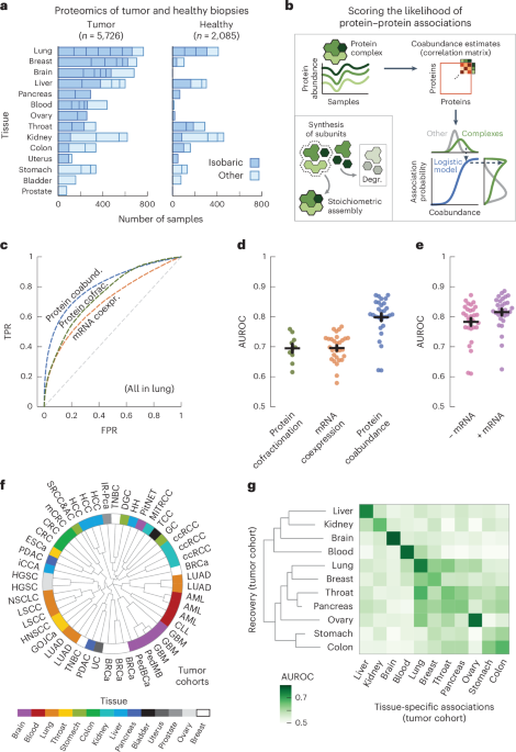
We started by collecting protein abundance data from proteomics studies of cohorts of participants with cancer. In total, we compiled a dataset of 50 studies across 14 human tissues, encompassing 5,726 samples of tumors and 2,085 samples of adjacent healthy tissue^{26,27,28,29,30,31,32,33,34,35,36,37,38,39,40,41,42,43,44,45,46,47,48,49,50,51,52,53,54,55,56,57,58,59,60,61,62,63,64,65,66,67,68,69,70,71,72,73,74,75} (Fig. 1a and Supplementary Table 1). We further included the mRNA expression data paired to the proteomics for 2,930 of the tumor and 722 of the healthy samples. Following previous studies, we used the fact that protein complex members are strongly transcriptionally and post-transcriptionally coregulated to compute probabilities of protein–protein associations from the abundance data^5,17,20 (Fig. 1b, Methods and Supplementary Fig. 1). In short, we preprocessed the abundance data to obtain a log-transformed and median-normalized abundance across participants. For each study, we then computed a coabundance estimate of a protein pair as the Pearson correlation when both proteins were quantified in at least 30 samples (Supplementary Fig. 2). Lastly, with pairs of subunits for curated stable protein complexes as ground-truth positives (CORUM⁷⁶), we used a logistic model for each study to convert the coabundance estimates to probabilities of protein–protein associations (Supplementary Figs. 3–5).

To test the ability of the association probabilities to recover known complex members, we computed receiver operating characteristic (ROC) curves for probabilities derived from protein coabundance, mRNA coexpression and protein cofractionation^6,7,77 (Fig. 1c). We found that protein coabundance (area under the curve (AUC) = 0.80 ± 0.01 (mean ± s.e.m.)) outperformed protein cofractionation (AUC = 0.69 ± 0.01) and mRNA coexpression (AUC = 0.70 ± 0.01) data for recovering known interactions (Fig. 1d and Methods). In addition, the combination of mRNA and protein abundance data did not significantly improve the recovery of known complex members (Fig. 1e; AUC = 0.82 ± 0.01, P = 0.15, according to a one-sided Welch’s t-test). Therefore, with roughly half of all cohorts having paired mRNA expression data available, we chose to only use protein coabundance for computing association probabilities. Additionally, we found similar AUCs when regressing gene expression out of the protein abundance before computing protein coabundance estimates (AUC = 0.78 ± 0.01, P = 0.18), suggesting that post-transcriptional processes but not regulation of gene expression drive most of the predictive power for protein associations.

Having established that the association probabilities derived from protein coabundance data recover known interactions of protein complex members, we sought to test whether replicate studies of the same tissue yielded association probabilities that were representative for each tissue. As a starting point, we used the gene expression data to establish that the association probabilities were not driven by cell-type composition⁷⁸ (Supplementary Fig. 6). Next, using the 1,115,405 association probabilities that were quantified for all studies, we found that the replicate cohorts from the same tissue generally clustered together (Fig. 1f; for example, blood, brain, liver and lung). Next, we selected the associations that were tissue specific, that is associations whose average probability exceeded the 95th percentile for a given tissue (0.68 ± 0.01 across tissues) and whose average probability remained below 0.5 across all other tissues. Through a hold-one-out methodology, we found that the tissue-specific associations were primarily recovered by cohorts of the same tissue of origin (AUC = 0.71 ± 0.01) compared to cohorts from different tissues (AUC = 0.56 ± 0.00, P < 0.05 for all tissues, according to a one-sided Welch’s t-test) (Fig. 1g, Methods and Supplementary Fig. 7). Together, these observations suggest that the tissue of origin is a major driver of differences between cohorts.

An atlas of protein associations in human tissues

With the replicate cohorts representing the tissue of origin, we aggregated the association probabilities from cohorts of the same tissue into single association scores for 11 human tissues (Fig. 2a and Methods). Aggregating the replicate cohorts was advantageous, as all but one of the individual cohorts were outperformed by the tissue-level scores for recovering known protein interactions (P = 1.3 × 10⁻⁹, according to a one-sided Welch’s t-test). Moreover, the tumor-derived scores outperformed the healthy-tissue-derived scores for all tissues (Fig. 2b; AUC = 0.87 ± 0.01 and 0.82 ± 0.01, respectively, P = 8.3 × 10⁻⁵, according to a one-sided Welch’s t-test). In addition to the biopsy, where the genetic heterogeneity of tumors increased variation between samples (Supplementary Fig. 8), we found several other factors affecting the recovery of known interactions, such as the available number of cohorts per tissue, the number of samples per cohort, the tissue of origin and the MS methodology (Supplementary Figs. 2 and 9). The healthy-tissue-derived and tumor-derived scores originated from separate dissections of the same tissues and participants and could, thus, serve as independent replicates. Analogous to the cohorts, we computed tissue-specific associations from the healthy-tissue-derived scores, which we then recovered with the tumor-derived scores (Fig. 2c). For all tissues, we found that the tumor-derived scores primarily recovered the tissue-specific associations of the same healthy tissue (AUC = 0.74 ± 0.02) compared to the other healthy tissues (AUC = 0.53 ± 0.01, P = 5.9 × 10⁻⁵, according to a one-sided Welch’s t-test). These analyses show that the coabundance-derived tissue-level association scores recover known protein interactions and are reproducible and representative of the tissue of origin (Supplementary Fig. 10).

We defined a protein association atlas with association scores for all quantified protein pairs by averaging the association probabilities over the cohorts of each tissue. The resulting association atlas scores the association likelihood for 116 million protein pairs across 11 human tissues (Fig. 2d). On average, each tissue contains association scores for 56 ± 6.2 million protein pairs, of which 10 ± 1.0 million are likely to be associated (score > 0.5, average accuracy = 0.81 over all tissues, recall = 0.73 and diagnostic odds ratio = 13.0) and 0.49 ± 0.08 million are ‘confident’ associations (score > 0.8, average accuracy = 0.99 across tissues, recall = 0.21 and diagnostic odds ratio = 31.9) (Supplementary Fig. 11). These protein associations tended to be likely and confident in only a few tissues, with 99,103 protein pairs having likely associations in all tissues (Fig. 2d and Supplementary Fig. 12).

Differences between tissues not driven by gene expression

One of the well-known drivers of differences in protein interactions between tissues is gene expression; proteins can interact only if their gene is expressed in a tissue. Indeed, the proteins that were quantified in a given tissue were generally enriched for genes with elevated expression for that same tissue but not the other tissues (Supplementary Fig. 13; P = 1.3 × 10⁻⁶, according to a one-sided Mann–Whitney U-test). However, only up to 7% of differences in (likely) associations between tissues can be explained by differences in gene expression and only through the lack of detection (Supplementary Fig. 14). These observations demonstrate that the likely associations for each tissue reflect but are not defined by differences in gene expression, further supporting our previous observation that protein coabundance is primarily driven by post-transcriptional processes.

Having established that association scores generally reproduce well and that differences between tissues are not driven by gene expression, we sought to measure the share of tissue-specific associations. To do so, we used a threshold association score to quantify the percentage of a tissue’s associations that were likely (score > 0.5) for the replicate (Fig. 2e, orange curve, comparing healthy-tissue-derived and tumor-derived replicates). As expected, we found that the percentage of likely associations increases with the threshold score, with 46.3% of likely associations and 90.2% of confident associations (score > 0.8) also being likely for the replicate tissue. Similarly, we found that these percentages decreased to 32.9% and 54.6%, respectively, when comparing associations between pairs of tissues from the association atlas (Fig. 2e, green curve). Lastly, depending on threshold scores, we found between 18.8% and 34.0% (interquartile range) of likely associations to be tissue specific between pairs of tissues, given the difference in probabilities between the curves for replicates and tissues. Therefore, with up to 7% of likely associations not quantified in other tissues because of gene expression (Supplementary Fig. 14), we estimated over 25.8% (18.8% + 7%) of likely associations to be tissue specific.

Tissues recover tissue-specific cellular components

We sought to characterize the likely associations that were shared between tissues. Compared to all likely associations (average Jaccard index = 0.19), we found that the similarity between pairs of tissues increased as we restricted the likely associations to interactions identified through high-throughput screens such as yeast two-hybrid (Jaccard index = 0.30; HuRI)³ or AP (Jaccard index = 0.41; BioPlex)⁴ experiments (Fig. 2f). Likewise, the similarity between pairs of tissues increased when restricting likely associations to known interactions reported for signaling (Jaccard index = 0.32; SIGNOR)⁷⁹, biological pathways (Jaccard index = 0.48; Reactome)⁸⁰, physical associations (Jaccard index = 0.56; STRING)⁸¹ or human protein complexes (Jaccard index = 0.74; CORUM)⁷⁶. Lastly, we found that the quantified differences and similarities between tissues were not sensitive to the choice of score cutoffs (Supplementary Fig. 15). Thus, known protein interactions are typically shared by the tissues in our association atlas, with signaling interactions being less commonly recovered between tissues than stable protein complexes. These observations reflect the divergence between tissues for different types of interactions and may also reflect differences in accuracy for recovering associations for stable protein complexes compared to spatiotemporal interactions that are dynamic.

Well-characterized protein complexes were generally preserved across tissues, becoming more variable as the complex-averaged association scores decreased (ρ = −0.77, P = 6.2 × 10⁻¹²⁵) (Supplementary Fig. 16). As seen in other proteomics datasets⁸², more variable complexes are typically involved signaling and regulation (for example, tumor necrosis factor and emerin), while more stable complexes are involved central cellular structures (for example, ribosomes and the respiratory chain) (Supplementary Fig. 16). While protein complexes varied little between tissues, we found that associations varied strongly for tissue-specific cellular components, for example, for the brain (synapse-related components), throat (structural components of muscle fiber), lung (motile cilia) and liver (peroxisomes) (Supplementary Fig. 17). This suggests that tissue-specific and cell-type-specific cellular components are an important driver of tissue-specific protein associations that are independent of simple expression differences.

Association atlas reveals cell-type-specific associations

To explore cell-type-specific associations in our association atlas, we took the AP2 adaptor complex as a well-known example. The AP2 complex has neuron-specific functions in addition to functions that are general to all cells⁸³. Indeed, the subunits of the AP2 complex were coabundant in all tissues (average association score between subunits = 0.80). We found 91 proteins that had association scores with all AP2 subunits in all tissues and were known to associate with AP2 (STRING score > 400). Among these, the 51 synaptic proteins (SynGO⁸⁴) had higher association scores with the AP2 complex in the brain (average score = 0.54) compared to the other tissues (average score = 0.48 ± 0.00, P = 6.7 × 10⁻⁶, according to a one-sided Mann–Whitney U-test). Conversely, the nonsynaptic interactors had lower association scores with the AP2 complex in the brain (average score = 0.33) compared to the other tissues (average score = 0.43 ± 0.00, P = 1.1 × 10⁻²¹, according to a one-sided Mann–Whitney U-test) (Fig. 3a). We explored further examples by focusing on cell-type-specific associations in the context of disease. We found that proteins of hemoglobin are related to anemia and have likely associations with anemia proteins but only in the blood (Fig. 3b and Methods). Likewise, we found that subunits of chylomicron, which transports dairy lipids from the intestines, contain and have likely associations with proteins related to Crohn’s disease but only in the colon^85,86. Lastly, we found that subunits of fibrinogen, synthesized in the liver, contain and have liver-only likely associations with proteins related to liver disease^87,88. For the other tissues, we could find many examples of tissue-specific and cell-type-specific associations for protein complexes, cellular components and disorders such as diabetes and asthma (Supplementary Fig. 18). These examples demonstrate that our association atlas can be used to study tissue-specific functions of protein complexes and context-dependent associations for disease genes.

Tissue-specific relations of traits and cellular components

We sought to generalize these examples of context-specific associations by systematically mapping the relationships amongst traits and multiprotein structures such as complexes or cellular components. As sets of proteins, we defined cellular components by Gene Ontology (GO) and defined human traits on the basis of the genome-wide association studies (GWAS) Open Targets (OTAR) locus-to-gene (L2G) score (≥0.5)^89,90,91. We then scored the relationship between sets of proteins with the median association score of all possible protein pairs between the sets (Fig. 3c, schematic, omitting the intersection between gene sets). In total, we scored the relationships between traits (107,306 pairs), between traits and cellular components (240,967 pairs) and between components (134,002 pairs) across all tissues (Fig. 3d and Supplementary Tables 2–4). The relationship scores that were high in all tissues were primarily of core cellular components such as the ribosome and spliceosome (72% of relationships with relative average score > 1.75), while the relationship scores that varied most across tissues often involved tissue-specific structures such as synaptic components (61% of relationships with a coefficient of variation (CV) > 0.4). These observations suggest that the relationship scores recapitulate the relatedness of protein sets in a tissue-specific manner, particularly for the brain.

Relationship scores for prioritizing disease genes

Additionally, we unbiasedly scored the tissue specificity of each protein set as the median association score between all pairs of its proteins (Methods and Supplementary Tables 5 and 6). Using these scores, we then selected the 15 traits most specific to the brain, 13 of which were indeed related to the brain (Supplementary Table 7). Clustering these traits using the trait–trait relationship scores from the brain revealed a hierarchical organization of traits with co-occurring conditions such as anorexia nervosa, obsessive–compulsive disorder (OCD) and Tourette syndrome closely clustering together^92,93 (Fig. 3e, left dendrogram). As an example, we further determined the 15 cellular components that had the strongest brain-specific relationships with OCD, all but one of which were related or specific to neurons (Fig. 3e, right dendrogram, and Methods). The majority of these cellular components had few genes in common with the genes confidently associated with OCD (Fig. 3e, orange heat map; Jaccard indices < 0.04). However, after removing the few genes confidently associated with OCD through GWAS, we found that almost all components were still enriched with or contained OCD-related genes (Fig. 3e, purple–green heat maps), that is, drug targets for OCD (odds ratio = 8.4 ± 1.8; ChEMBL clinical stage 2 or higher)⁹⁴, genes related to OCD from mouse deletion phenotypes (odds ratio = 4.8 ± 0.8; International Mouse Phenotyping Consortium (IMPC) score ≥ 0.5)⁹⁵ or genes less confidently linked to OCD through GWAS (odds ratio = 1.6 ± 0.2, OTAR L2G score < 0.5) (Methods). Moreover, these 15 components with the strongest OCD relationships in the brain were more strongly enriched with OCD-related genes than other cellular components that contained OCD-linked genes (P = 4.3 × 10⁻¹¹ (drug targets), 3.4 × 10⁻¹⁵ (genes related to OCD in mice) and 6.6 × 10⁻⁷ (genes less confidently linked to OCD through GWAS), according to one-sided Mann–Whitney U-tests).

Together, the results above demonstrate that the proposed relationship scores can prioritize cellular components that are enriched with trait-relevant genes. Analogously, we found that we could use the relationship scores for reconstructing the hierarchical organization of the cell, including maps of subcellular structures and modules of tissue-specific relations between cellular components (Supplementary Fig. 19). These observations demonstrate the potential for our association atlas to facilitate the systematic mapping of relations among traits, cellular compartments and likely other ontology terms.

Validated brain interactions for schizophrenia-related genes

The results above indicate that the tissue-specific associations could facilitate the prioritization of disease-linked genes by functional association. Indeed, direct interactors of disease-linked genes have been used to prioritize causal genes in genetically linked loci and shown to be enriched in successful drug candidates^96,97,98. To explore this in more detail, we constructed a network of brain interactions for schizophrenia (SCZ)-related genes. Specifically, we sought to prioritize highly ranked associations for the brain that involve SCZ-related genes and that have additional evidence from orthogonal methodologies.

We started by taking n = 369 genes associated with SCZ through GWAS studies (‘starting genes’, L2G scores ≥ 0.5) and computed the top 25 traits and cellular components that had the strongest tissue-specific relation to SCZ in each tissue (Fig. 4a and Methods). This gave us a collection of genes related to SCZ in a tissue-specific manner. For each tissue, we then filtered for protein pairs that had one SCZ starting gene and one SCZ-related gene and required these protein pairs to have association scores exceeding the 97th percentile of the tissue scores (association score = 0.70 ± 0.01, 0.73 in the brain), leading to tissue-specific networks of associations for SCZ-related genes (Supplementary Fig. 20 and Supplementary Table 8). After removing the SCZ starting genes from the brain network, the remaining genes were still enriched for genes associated with SCZ in mice (Benjamini–Hochberg (BH)-adjusted P value = 1.5 × 10⁻⁵, IMPC score ≥ 0.5), drug targets for SCZ (BH-adjusted P value = 9.8 × 10⁻⁵, ChEMBL clinical stage 2 or higher) and other variants associated with SCZ (BH-adjusted P value = 1.0 × 10⁻⁷, OTAR L2G scores < 0.5), according to one-sided Fisher exact tests. This enrichment was specific to the brain compared to any of the other tissues, suggesting that the proposed methodology presents a systematic approach for prioritizing disease genes of tissue-specific traits (Fig. 4b).

Indeed, for brain-related disorders, including autism, attention deficit hyperactivity disorder (ADHD), Tourette syndrome and others, we found that the proposed methodology of prioritizing protein associations for disease-linked genes enriched, specifically in the brain, for other genes associated with the respective disorder through mouse phenotypes or drug targets, with many also being enriched for GWAS variants that are less confidently linked to the disorder (Supplementary Fig. 21).

Having established that the presented methodology prioritizes protein associations that enrich for disease-related genes in a tissue-specific manner, we sought to validate the prioritized protein associations through additional evidence. Specifically, to further validate the networks of predicted associations for SCZ-related genes, we assembled a curated dataset of brain interactions established experimentally through pulldowns using human brain cells (that is, AP–MS or coimmunoprecipitation–MS in human microdissected brain tissue or human induced pluripotent stem cell-derived neurons^{99,100,101,102,103}). This dataset contained 7,887 human brain interactions for 30 bait proteins and has been incorporated into the IntAct database⁹ (Supplementary Table 9). We filtered these brain interactions for the bait proteins that were associated with SCZ (OTAR L2G score ≥ 0.5) and further filtered the tissue-specific networks of SCZ-related genes for associations involving at least one bait protein. The remaining associations of SCZ-related genes were strongly enriched with the interactions from pulldowns with SCZ-related baits, especially for the brain (log BH-adjusted P value = 84.3, according to a one-sided Fisher exact test) compared to the other tissues (log BH-adjusted P value = 1.8 on average) (Fig. 4c). Thus, the brain associations of SCZ-related genes but not the other tissues were experimentally validated by pulldown studies and enriched with SCZ-related association partners.

Next, we filtered the prioritized brain associations for SCZ-related genes for interactions that were also found through the pulldown studies to obtain a network of 205 validated brain interactions for SCZ-related genes (average association scores = 0.86 in the brain), which we simplified to only show synaptic (SynGO) genes having prior evidence (Fig. 4d, Methods and Supplementary Table 10). The visualized network contained 56 proteins connected to three bait proteins through a collection of 66 validated brain interactions. These connected proteins included SCZ drug targets (3 proteins; clinical stage 2 or higher), proteins associated with SCZ in mice (12 proteins; IMPC score ≥ 0.5) or proteins linked with SCZ with weaker prior evidence (15 proteins; OTAR L2G scores < 0.5). Surprisingly, only four of the visualized brain interactions were confidently reported in any of the major protein interaction databases before our curation effort (CACNA1C with CACNB1, CACNB2 and CACNB4 (STRING scores > 750) and SRC (Signor)) and only the interactions of SHANK3 with AP2B1 and CLTB were quantified in more than three other tissues (association scores = 0.34 ± 0.08 and 0.29 ± 0.04 in the other tissues). These observations support our earlier analysis that the network of validated interactions of SCZ-related genes is specific to the brain.

The visualized network contained several groups of highly interconnected proteins (STRING scores > 750). These groups were enriched with genes of cellular components typical for neuronal functioning and SCZ, such as a group of proteins for the postsynaptic cytoskeleton¹⁰⁴ (BH-adjusted P value = 2.3 × 10⁻⁸) or for clathrin-coated vesicles (9.4 × 10⁻¹⁴), according to one-sided Fisher exact tests. For the clathrin vesicle coat, the network connected all subunits of the AP2 complex and clathrin proteins to HCN1. Interestingly, previous pulldown studies showed that HCN channels directly interact with TRIP8b (refs. ^105,106). TRIP8b regulates the trafficking of HCN channels¹⁰⁶ and mainly associates with the AP2 complex¹⁰⁷. Moreover, while AP2 and clathrin are not cell type specific, both HCN1 and TRIP8b were found to be enriched at parvalbumin (PV)-positive synapses¹⁰⁸, with HCN channels being specific to PV neurons and important for their high firing frequencies^109,110. Given the link of PV neurons with SCZ^{111,112,113,114,115}, these observations suggest that AP2 and clathrin may be involved in a PV neuron-specific disruption of HCN channel trafficking with SCZ.

To suggest putative interface models for the validated brain interactions for SCZ-related genes, we used AlphaFold2 to predict the structures for 205 protein interactions, including the entire visualized network (Fig. 4d and Supplementary Table 11). The predicted models had more confident interactions compared to models for known complex members from CORUM¹¹⁶ (average pDockQ scores = 0.20 and 0.13, respectively, P = 1.6 × 10⁻¹⁹, according to a one-sided Mann–Whitney U-test). In total, we identified 15 moderate-confidence interactions (interface predicted template modeling (ipTM) scores > 0.5). These included the brain-specific binding of all three 14-3-3 proteins (YWHAG, YWHAH and YWHAZ) with HCN1 (Fig. 4e; average association score = 0.82, average ipTM score = 0.65). The interfaces of these three models overlap and are located in the C-terminal disordered region of HCN1 (residues 775–802). This consensus interface includes a predicted 14-4-3-binding site (centered around S789; average ipTM score = 0.75 at the putative binding site, 14-3-3-Pred score = 0.457)¹¹⁷ that has been verified through pulldown experiments¹¹⁸. Indeed, the binding of 14-3-3 proteins with HCN1 was found to be dependent on the phosphorylation of S789, with the interaction between 14-3-3 and HCN1 likely inhibiting HCN1 degradation¹¹⁸.

Lastly, the network contained 15 genes within loci genetically associated with SCZ that had weaker evidence supporting them as the causal genes at each locus. Given their interaction with other SCZ-related genes, these could be prioritized as more likely causal because of their functional roles. Some of these genes (AP2B1, ATP2B2 and SYNGAP1) had the highest L2G score for their respective locus with single-nucleotide polymorphisms (SNPs) linked to SCZ but had scores below the 0.5 cutoff used (0.457, 0.264 and 0.251, respectively)^90,91. In addition to the AP2 complex, we found a member of the AP3 complex (AP3B2). AP3B2 had the second highest score for the locus with SNPs (rs783540), which had splicing and expression quantitative trait locus (QTL) associations with AP3B2 but was ranked higher for disruption of CPEB1 given that the variant lies within a CPEB1 intron. Similarly, MARK2 was ranked second for two SNPs (rs7121067 and rs11231640), both having splicing and promoter capture Hi-C associations with MARK2 but being ranked higher for disrupting RCOR2 because of proximity to its transcription start site. CDC42 and NTRK2 had the second highest L2G scores for their locus but the top associated genes (WNT4 and AGTPBP1, respectively) had lower and less specific expression in the brain¹².

Cofractionation-derived synapse-specific interactome

As a final application of our protein association atlas, we focused on the interactome of synapses. To do so, we prepared and purified synaptosomes from rat brains as an orthogonal approach for validating the brain associations. We fractionated the synaptosomes with size-exclusion chromatography (SEC) into 75 fractions that were then subjected to liquid chromatography (LC)–MS/MS. A total of 3,409 unique proteins were detected, including well-known protein complexes such as the CCT complex subunits, whose profiles correlate across the fractions (Fig. 5a; average correlation coefficient = 0.96).

We preprocessed the fractionation profiles of the synaptosome and computed the coabundance of proteins across fractions to score the cofractionation of 4,276,350 protein pairs in rat synapses (Methods). To increase the confidence of the interaction scores, we then combined the rat synaptosome with other cofractionation profiles from in vivo mouse brains⁶ and subcellular fractionation profiles from human glioblastoma cells⁷. We merged the cofractionation studies by orthologs that were quantified in all three datasets and computed interaction probabilities with a logistic model using the CORUM database as positives (Methods and Supplementary Table 12). The resulting synaptic interactome quantified 1,309,771 interaction probabilities for 1,619 proteins and improved the recovery of known interactions compared to the cofractionation studies individually (Fig. 5b; AUC = 0.80 and 0.72). Of the 1,619 proteins in the interactome, 24% are annotated as synaptic proteins in the SynGO database, 49% have been reported as synapse-enriched in mouse brains and 56% have previously been identified through crosslinking MS (XL-MS) of the mouse synaptosome^84,108,119. All XL-MS interactions for these proteins were quantified in our synaptic interactome, having association scores of 0.59 compared to 0.37 for other associations (P = 2.0 × 10⁻⁴⁴, according to a one-sided Mann–Whitney U-test). Moreover, the synaptic interactions between synapse-enriched proteins were more likely compared to other interactions (average association scores = 0.40 and 0.36, P < 1 × 10⁻³⁰⁰, according to a one-sided Mann–Whitney U-test). Together, these observations suggest that our synaptic interactome largely aligns with current state-of-the-art synaptic interaction resources and scores the likelihood of interactions for a wide range of synaptic proteins, with interactions being more likely for synaptic proteins compared to other proteins.

Validated synaptic interactions for brain disease genes

The interactions between synapse-enriched proteins formed more likely associations compared to associations of nonsynaptic proteins, especially for the brain compared to the other tissues of our association atlas (Fig. 5c). Given this brain-specific elevated likelihood of synaptic interactions, we constructed a network of interactions between synaptic proteins (in SynGO or synapse-enriched in mouse brains) that were both likely coabundant in the brain (109,913 associations) and likely cofractionated for the synaptosome (121,732 interactions). The resulting network consisted of a collection of 37,318 validated protein interactions between synaptic proteins (Supplementary Table 13). These synaptic interactions were primarily specific to the brain because few of the interactions were likely for the majority of other tissues in our association atlas (20%) and only a small fraction have been reported in any protein interaction database (5.8% in STRING, 1.3% in HuMAP, 3.6% in IntAct and 1.6% in BioPlex).

We were particularly interested in the validated interactions of synaptic proteins that are associated with brain disorders. As before, we filtered for GWAS traits that had associated genes through mouse phenotyping (IMPC) or known drug targets (ChEMBL) and whose trait-level association scores were elevated in the brain compared to the other tissues (z score > 1; Methods). We found that 10 of the resulting 13 traits were disorders clearly related to the brain and selected the 727 confident synaptic interactions between genes associated with these brain-specific traits (association scores = 0.7 and 0.81 on average in the synaptosome and brain, respectively). Additionally, to suggest putative interface models, we used AlphaFold2 to predict the structures for these 727 interactions. The predicted models had more confident interactions compared to models for known interactors in CORUM (average pDockQ scores = 0.28 and 0.13, P = 3.7 × 10⁻¹⁴⁷, according to a one-sided Mann–Whitney U-test) or HuMAP (pDockQ scores = 0.28 and 0.25, P = 2.4 × 10⁻¹⁷) and high-confidence models (ipTM scores > 0.7) were enriched for additional evidence from XL-MS experiments in mouse synaptosomes¹¹⁹ (Supplementary Fig. 22). In total, we identified 105 moderate-confidence interactions (ipTM scores > 0.5; Supplementary Table 14). Lastly, we visualized (simplified) the networks of validated synaptic interactions between trait-related genes of the brain disorders (Fig. 5d and Methods).

Prioritizing synaptic disease genes for brain disorders

Several genes in the networks had weaker prior evidence supporting them as the causal genes at loci genetically associated with the brain disorders. These genes could be prioritized as more likely to be causal for the disorders because of their validated synaptic interactions with other genes that were confidently associated with the same disorders. As before, we looked for genes with the highest (below cutoff) L2G scores for their respective loci with SNPs linked to the brain disorders. We found likely causal genes for ADHD (MDH1, score = 0.491; CADPS2, score = 0.340; PIK3C3, score = 0.323), SCZ (TOM1L2, score = 0.492; AP2B1, score = 0.457; PSD3, score = 0.429; MYO18A, score = 0.428; ATP2B2, score = 0.264; TMX2, score = 0.232), Alzheimer disease (CLPTM1, score = 0.378; MADD, score = 0.315), autism (ATP2B2, score = 0.264; ATP2A2, score = 0.243), unipolar depression (MADD, score = 0.244) and bipolar disorder (ATP2A2, score = 0.206), with the last variant (MYO18A, score = 0.428) additionally being likely causal for Tourette syndrome, OCD, ADHD and unipolar depression^90,91. Of these genes, all but ATP2A2, MDH1, MYO18A and PIK3C3 had the highest or second highest expression in brain tissue¹².

Additionally, we found genes with synaptic interactions that did not have the highest L2G score for the respective SNP linked to the brain disorders but still had additional evidence. For example, we found that PAFAH1B1 associated with RHOA in our synaptic interactome, with both having weak prior evidence for being causal to depression. PAFAH1B1 has a role in neural mobility and is required for activation of Rho guanosine triphosphatases such as RhoA¹²⁰. PAFAH1B1 was the second highest scoring gene for the locus with an SNP (rs12938775) linked to unipolar depression. This variant has expression QTL associations with PAFAH1B1 and lies within a PAFAH1B1 intron, despite being more distant to the transcription start site of PAFAH1B1 compared to the highest scoring gene (CLUH). However, PAFAH1B1 encodes a synaptic protein, whereas CLUH does not, with the expression of PAFAH1B1 being higher and more specific to the brain compared to CLUH¹². Overall, this example demonstrates how orthogonal approaches targeting subcellular structures and individual tissues can provide tissue-specific protein interaction networks and aid in the prioritization of genes likely to be causal for tissue-related disorders.